In our previous post, we discussed local sensitivity and how we can get accuracy guarantees that scale with local sensitivity, which can be much better than the global sensitivity guarantees attained via standard noise addition mechanisms. In this post, we will look at what we can do when even the local sensitivity is unbounded. This is obviously a challenging setting, but it turns out that not all hope is lost.

As a motivating example, suppose we have a dataset \(x=(x_1,x_2,\cdots,x_n)\) and we want to approximate \(\max_i x_i \) in a differentially private manner. The difficulty is that adding a single element to \(x\) can increase the maximum arbitrarily. That is, if \(x’=(x_1,x_2,\cdots,x_n,\infty)\), then \(\max_i x’_i=\infty\). Differential privacy requires us to make the outputs \(M(x)\) and \(M(x’)\) indistinguishable, which seems to directly contradict our accuracy goal \(M(x) \approx \max_i x_i\).

One solution to the problem of unbounded sensitivity is to clip the inputs, so that the sensitivity becomes bounded. But this requires knowing a good a priori approximate upper bound on the \(x_i\)s. Trying to find such an upper bound is probably the very reason we want to approximate the maximum in the first place!

Another solution is to “aim lower:” Instead of aiming to approximate the largest element \(x_{(n)} := \max_i x_i\), we can aim to approximate the \(k\)-th largest element \(x_{(n-k+1)}\). The \(k\)-th largest element has bounded local sensitivity, which means we can apply the inverse sensitivity mechanism or similar tools. And – spoiler alert – this is essentially what we will do. However, we will present an algorithm that is more general than just for approximating the maximum.

The algorithm we present is due to Fang, Dong, and Yi [FDY22]. In terms of applications, a natural setting where we may need to approximate functions of unbouned local sensitivity is when each person can contribute multiple items to the dataset. This setting is often referred to as “user-level differential privacy” or “user DP.”¹ For example, if we have a collection of web browsing histories, we may wish to estimate the total number of webpages visited; this has unbounded local sensitivity because a single person could visit an arbitrary number of webpages.

Down Sensitivity

Observe that, while adding one element to the input can increase the maximum arbitrarily, removing one element can only decrease it by the gap between the largest and second-largest elements \(x_{(n)}-x_{(n-1)}\). In other words, the maximum satisfies some kind of one-sided local sensitivity bound. This is the general property we will rely on.

We define the \(k\)-down sensitivity² of the function \(f : \mathcal{X}^* \to \mathbb{R}\) at the input \(x\in\mathcal{X}^*\) as \[\mathsf{DS}^k_f(x) := \sup_{x’ \subseteq x : \mathrm{dist}(x,x’) \le k} |f(x)-f(x’)|. \tag{1}\] Here \(\mathrm{dist} : \mathcal{X}^* \times \mathcal{X}^* \to \mathbb{R}\) is the size of the symmetric difference between the two input tuples/multisets \(\mathrm{dist}(x,x’) = |x \setminus x’| + | x’ \setminus x |\), which defines a metric. In other words, it measures how many people’s data must be added or removed to get from one dataset to the other. For comparison, the local sensitivity is \[\mathsf{LS}^k_f(x) := \sup_{x’\in\mathcal{X}^* : \mathrm{dist}(x,x’) \le k} |f(x)-f(x’)|. \tag{2}\] The difference between Equations 1 and 2 is simply that down sensitivity only considers removing elements from \(x\), while local sensitivity considers both addition and removal. Thus, the down sensitivity is at most the local sensitivity, which is, in turn, upper bounded by the global sensitivity: \(\mathsf{DS}^k_f(x) \le \mathsf{LS}^k_f(x) \le k \cdot \mathsf{GS}_f\).

Intuitively, what is nice about down sensitivity is that it only considers the actual data we have at hand. It doesn’t consider any hypothetical people’s data that could be added to the dataset. It is appealing to only have to deal with “real” data.

Our goal now is to estimate \(f(x)\) in a differentially private manner, where the accuracy guarantee scales with the down sensitivity.

Monotonicity Assumption

In order to do anything, we need some assumptions about the function \(f : \mathcal{X}^* \to \mathcal{Y}\) that we are trying to approximate. First we will assume that \(\mathcal{Y} \subseteq \mathbb{R}\) is finite and \(f\) is surjective.³ The main assumption is monotonicity: \[\forall x’ \subseteq x \in \mathcal{X}^* ~~~ f(x’) \le f(x). \tag{3}\] The maximum and many other example functions satisfy this assumption.

Intuitively, we need this assumption to ensure that the down sensitivity is well-behaved. Specifically, Lemma 1 below requires monotonicity.

As an example of what could happen if we don’t make this assumption, consider the function \(\mathrm{sum}(x) := \sum_i x_i\) and the pair of neighbouring inputs \(x=(1,1,\cdots,1)\in\mathcal{Y}^n,x’=(1,1,\cdots,1,-100n)\in\mathcal{Y}^{n+1}\). Then, for all \(1 \le k\le n\), we have \(\mathsf{DS}_{\mathrm{sum}}^k(x)=k\), but \(\mathsf{DS}_{\mathrm{sum}}^k(x’)=100n\).

Note that the sum is monotone if we restrict to non-negative inputs. In general, we can take any function \(g\) and convert it into a monotone function \(f\) by defining \(f(x) = \max\{ g(\check{x}) : \check{x} \subseteq x \}\). Depending on the context, this \(f\) may or may not be a good proxy for \(g\).

A Loss With Bounded Global Sensitivity

Given a monotone function \(f : \mathcal{X}^* \to \mathbb{R}\), we define a loss function \(\ell : \mathcal{X}^* \times \mathbb{R} \to \mathbb{Z}_{\ge 0}\) by \[\ell(x,y) := \min\{ \mathrm{dist}(x,\tilde{x}) : \tilde{x} \subseteq x, f(\tilde{x}) \le y \}. \tag{4}\] In other words, \(\ell(x,y)\) measures how many entries of \(x\) we need to remove to decrease the function value until \(f(x) \le y\). Yet another way to think of it is that \(\ell(x,y)\) is the distance from the point \(x\) to the set \(f^{-1}((-\infty,y]) \cap \{ \tilde{x} : \tilde{x} \subseteq x \} \).

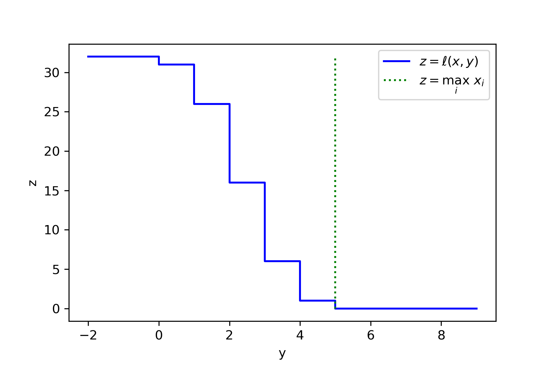Figure 1: Visualization of the loss \(\ell(x,y)\) corresponding to \(f(x)=\max_i x_i\) for a dataset representing the distribution \(\mathrm{Binomial}(5,1/2)\) i.e. the true maximum is \(5\) and the dataset is \(x=(0,\underbrace{1,1,1,1,1}_{5\times},\underbrace{2,2,\cdots,2}_{10\times},\underbrace{3,3,\cdots,3}_{10\times},\underbrace{4,4,4,4,4}_{5\times},5)\).

The key property we need is that this loss has bounded sensitivity. We split the proof into Lemmas 1 and 2.

Lemma 1. Let \(f : \mathcal{X}^* \to \mathbb{R}\) satisfy the monotonicity property in Equation 3. Define \(\ell : \mathcal{X}^* \times \mathbb{R} \to \mathbb{Z}_{\ge 0}\) as in Equation 4.
Let \(x’ \subseteq x \in \mathcal{X}^*\). Then \(\ell(x’,y)\le\ell(x,y)\) for all \(y \in \mathbb{R}\).

Proof. Fix \(y \in \mathbb{R}\) and \(x’ \subseteq x \in \mathcal{X}^*\). Let \(x_\Delta = x \setminus x’ \subseteq x\), so that \(x’ = x \setminus x_\Delta \).

Let \(\widehat{x} \subseteq x\) satisfy \(f(\widehat{x})\le y\) and \(\mathrm{dist}(x,\widehat{x})=\ell(x,y)\). Define \(\widehat{x}’ = \widehat{x} \setminus x_\Delta\). This ensures \(\widehat{x}’ \subseteq x’\) and \[\mathrm{dist}(x’,\widehat{x}’) = \mathrm{dist}(x \setminus x_\Delta , \widehat{x} \setminus x_\Delta ) \le \mathrm{dist}(x,\widehat{x}).\]

By monotonicity, \(f(\widehat{x}’) \le f(\widehat{x}) \le y\). Thus \[\ell(x’,y) = \min\{ \mathrm{dist}(x’,\tilde{x}’) : \tilde{x}’ \subseteq x’, f(\tilde{x}’) \le y \}\]\[ \le \mathrm{dist}(x’,\widehat{x}’) \le \mathrm{dist}(x,\widehat{x}) = \ell(x,y).\] ∎

Lemma 2. Let \(f : \mathcal{X}^* \to \mathbb{R}\). Define \(\ell : \mathcal{X}^* \times \mathbb{R} \to \mathbb{Z}_{\ge 0}\) as in Equation 4.
Let \(x’ \subseteq x \in \mathcal{X}^*\). Then \(\ell(x,y)\le\ell(x’,y)+\mathrm{dist}(x,x’)\) for all \(y \in \mathbb{R}\).

Proof. Fix \(y \in \mathbb{R}\) and \(x’ \subseteq x \in \mathcal{X}^*\).

Let \(\widehat{x}’ \subseteq x’\) satisfy \(f(\widehat{x}’)\le y\) and \(\mathrm{dist}(x’,\widehat{x}’)=\ell(x’,y)\). Since \(\widehat{x}’ \subseteq x’ \subseteq x\), we have \[\ell(x,y) = \min\{ \mathrm{dist}(x,\tilde{x}) : \tilde{x} \subseteq x, f(\tilde{x}) \le y \} \le \mathrm{dist}(x,\widehat{x}’) \]\[ \le \mathrm{dist}(x,x’) + \mathrm{dist}(x’,\widehat{x}’) = \ell(x,y)+\mathrm{dist}(x,x’),\] by the triangle inequality, as required. ∎

Note that we only needed the monotonicity assumption for Lemma 1. Combining the two lemmas gives \[ \forall x’ \subseteq x ~ \forall y ~~~~~ \ell(x’,y) \le \ell(x,y) \le \ell(x’,y) + \mathrm{dist}(x,x’).\] Overall we have the following guarantee.

Proposition 3. (Global Sensitivity of the Loss) Let \(f : \mathcal{X}^* \to \mathbb{R}\) satisfy the monotonicity property in Equation 3. Define \(\ell : \mathcal{X}^* \times \mathbb{R} \to \mathbb{Z}_{\ge 0}\) as in Equation 4.
Then, for all \(x, x’ \in \mathcal{X}^*\) and all \(y \in \mathbb{R}\), we have \[|\ell(x,y)-\ell(x’,y)| \le \mathrm{dist}(x,x’).\]

Proof. Fix \(x, x’ \in \mathcal{X}^*\) and \(y \in \mathbb{R}\). Let \(x’’ = x \cap x’\). Since \(x’’ \subset x’\) and \(f\) is assumed to be monotone, Lemma 1 gives \(\ell(x’’ ,y) \le \ell(x’,y)\). Also \(x’’ \subset x\), whence Lemma 2 gives \(\ell(x,y) \le \ell(x’’ , y) + \mathrm{dist}(x , x’’ )\). Note that \( \mathrm{dist}(x , x’’ ) = | x \setminus x’’ | = | x \setminus x’ | \le \mathrm{dist}(x , x’ ).\) Combining inequalities gives \(\ell(x,y) \le \ell(x’ , y) + \mathrm{dist}(x , x’ )\). The other direction is symmetric. ∎

The Shifted Inverse Sensitivity Mechanism

Let’s recap where we are: We have a monotone function \(f : \mathcal{X}^* \to \mathcal{Y}\), where \(\mathcal{Y} \subseteq \mathbb{R}\) is finite. We want to approximate \(f(x)\) privately. Equation 4 gives us a loss \(\ell\) that is low-sensitivity. We have \(\ell(x,f(x))=0\) and, if \(y < f(x)\) decreases, the loss \(\ell(x,y)\) increases (depending on the down sensitivity of \(f\)). So far, so good. The problem is that if \(y > f(x)\) increases, the loss \(\ell(x,y)\) doesn’t increase. This means we can’t just throw this loss into the exponential mechanism.

Intuitively, the way we get around this problem is by looking for a value \(y\) such that the loss \(\ell(x,y)\) is greater than zero, but not too large. That is, we “shift” our goal from trying to minimize \(\ell(x,y)\) to minimizing something like \(|\ell(x,y)-\tau|\) for some integer \(\tau>0\). Going back to the example of the maximum, this corresponds to aiming for the \((\tau+1)\)-th largest value instead of the largest value. The hope is that we get an output with \(|\ell(x,y)-\tau|<\tau\), which for the maximum example corresponds roughly to getting a value between the largest value and the \(2\tau\)-th largest value.

Fang, Dong, and Yi [FDY22] directly apply the exponential mechanism [MT07] with a loss of the form \(|\ell(x,y)-\tau|\).⁴ This yields the following guarantee.

Theorem 4. (Shifted Inverse Sensitivity Mechanism) Let \(f : \mathcal{X}^* \to \mathcal{Y}\) be monotone (Equation 3), where \(\mathcal{Y} \subseteq \mathbb{R}\) is finite. Let \(\varepsilon>0\) and \(\beta \in (0,1)\). Then there exists an \(\varepsilon\)-differentially private \(M : \mathcal{X}^* \to \mathcal{Y}\) with the following accuracy guarantee. For all \(x \in \mathcal{X}^*\), we have \[\mathbb{P}\left[ f(x) \ge M(x) \ge f(x) - \mathsf{DS}_f^{2\tau}(x) \right] \ge 1 - \beta,\] where \(\tau=\left\lceil\frac{2}{\varepsilon}\log\left(\frac{|\mathcal{Y}|}{\beta}\right)\right\rceil\).

This is exactly the kind of guarantee we were aiming for; the accuracy scales with the down sensitivity, which could be much smaller than either the local sensitivity or the global sensitivity. Note that the guarantee gives an underestimate: \(M(x) \le f(x)\). This is inherent. If the function has infinite “up sensitivity,” then we cannot give an upper bound in a differentially private manner.

The shifted inverse sensitivity mechanism has the same limitations as the inverse sensitivity mechanism that we discussed in our previous post. Namely, computing the loss can be computationally intractable for general functions and we have a \(\log|\mathcal{Y}|\) dependence. (We will discuss how to improve this next.) An additional limitation is that we need the monotonicity assumption. But, as discussed earlier, down sensitivity behaves weirdly without this assumption.

Beyond the Exponential Mechanism

Applying the exponential mechanism to find \(y\) with \(\ell(x,y)\approx\tau\) yields a clean guarantee in Theorem 4. However, there are other methods we can apply which may be simpler⁴ and give better asymptotic guarantees.

Observe that the loss \(\ell(x,y)\) is a decreasing function of \(y\). The exponential mechanism does not exploit this structure. A very natural alternative algorithm is to perform binary search.⁵

We describe the algorithm in pseudocode and briefly analyze it: The input is the loss \(\ell\) defined in Equation 4, the dataset \(x\), an ordered enumeration of the set of outputs \(\mathcal{Y} = \{y_0 \le y_1 \le \cdots \le y_{|\mathcal{Y}|-1} \}\), and parameters \(\sigma,\tau>0\).

def noisy_binary_search(loss, x, Y, sigma, tau):
     i_min = 0
     i_max = len(Y) - 1
     while i_min + 1 < i_max:
          k = (i_min + i_max) // 2
          v = loss(x, Y[k]) + laplace(sigma)
          if v <= tau:
               i_max = k
          else:
               i_min = k
     return Y[i_max]

Since each iteration satisfies \(\frac1\sigma\)-differential privacy and there are at most \(\lceil \log_2 |\mathcal{Y}| \rceil-1\) iterations, the algorithm satisfies \(\varepsilon\)-differential privacy for \(\varepsilon = \frac{\log_2 |\mathcal{Y}|}{\sigma} \) by basic composition. Alternatively, using advanced composition, we see that the algorithm satisfies \(\rho\)-zCDP [BS16] for \(\rho = \frac{\log_2 |\mathcal{Y}|}{2\sigma^2} \).

By a union bound, each noise sample has magnitude at most \(\tau\) with probability at least \(1 - \exp(-\tau/\sigma) \cdot \log_2|\mathcal{Y}|\).⁶ Assuming the noise magnitudes are \(\le\tau\), the binary search maintains the invariants \(\ell(x,y_{i_\min})>0\) and \(\ell(x,y_{i_\max})\le 2\tau\). These invariants imply \(y_{i_\min} < f(x)\) and \(y_{i_\max} \ge f(x) - \mathsf{DS}_f^{2\tau}(x)\) respectively. At the end of the binary search, \(i_\min+1 \ge i_\max\) and thus \(y_{i_\min} < f(x)\) implies \(y_{i_\max} \le f(x)\).

Setting \(\tau = \sigma \cdot \log\left(\frac{\log_2|\mathcal{Y}|}{\beta}\right)\) and \(\sigma = \frac{\log_2|\mathcal{Y}|}{\varepsilon}\) yields a result similar to Theorem 4.

Setting \(\tau = \sigma \cdot \log\left(\frac{\log_2|\mathcal{Y}|}{\beta}\right)\) and \(\sigma = \sqrt{\frac{\log_2|\mathcal{Y}|}{2\rho}}\) yields the following result for concentrated differential privacy [DR16,BS16]. Note that setting \(\rho = \frac{\varepsilon^2}{4\log(1/\delta)+4\varepsilon}\) suffices to give \((\varepsilon,\delta)\)-differential privacy [e.g. S22 Remark 15].

Theorem 5. (Shifted Inverse Sensitivity Mechanism with Concentrated Differential Privacy) Let \(f : \mathcal{X}^* \to \mathcal{Y}\) be monotone (Equation 3), where \(\mathcal{Y} \subseteq \mathbb{R}\) is finite. Let \(\rho>0\) and \(\beta \in (0,1)\). Then there exists an \(\rho\)-zCDP \(M : \mathcal{X}^* \to \mathcal{Y}\) with the following accuracy guarantee. For all \(x \in \mathcal{X}^*\), we have \[\mathbb{P}\left[ f(x) \ge M(x) \ge f(x) - \mathsf{DS}_f^{2\tau}(x) \right] \ge 1 - \beta,\] where \(\tau = \sqrt{\frac{\log_2|\mathcal{Y}|}{2\rho}} \cdot \log\left(\frac{\log_2|\mathcal{Y}|}{\beta}\right) \).

Comparing Theorems 4 and 5 we see an asymptotic improvement in the dependence on the size of the output space \(|\mathcal{Y}|\). (This improvement is the benefit of advanced composition.) Theorem 4 gives \(\tau = \Theta(\log|\mathcal{Y}|)\), while Theorem 5 gives \(\tau = \Theta(\sqrt{\log|\mathcal{Y}|} \cdot \log \log |\mathcal{Y}|)\).⁷ In exchange, Theorem 4 gives a pure differential privacy guarantee (i.e. \((\varepsilon,\delta)\)-DP with \(\delta=0\)), while Theorem 5 gives a concentrated differential privacy guarantee, which can be translated to approximate differential privacy (i.e. \((\varepsilon,\delta)\)-DP with \(\delta>0\)).

We can actually do even better than binary search! The problem we’re solving with binary search is actually an instance of the generalized interior point problem [BDRS18] (which is essentially the same as quasi-concave optimization [CLNSS23]). This problem and its variants have been extensively studied in the context of private learning [BNS13,BNSV15,etc.] The upshot is that, under \((\varepsilon,\delta)\)-differential privacy, we can achieve the same result as Theorems 4 and 5 with \(\tau = \frac{\log(1/\delta)}{\varepsilon} \cdot 2^{O(\log^* |\mathcal{Y}|)}\), where \(\log^*\) denotes the iterated logaritm.

Theorem 6. (Shifted Inverse Sensitivity Mechanism with Approximate Differential Privacy) Let \(f : \mathcal{X}^* \to \mathcal{Y}\) be monotone (Equation 3), where \(\mathcal{Y} \subseteq \mathbb{R}\) is finite. Let \(\varepsilon>0\) and \(\delta \in (0,.1)\). Then there exists an \((\varepsilon,\delta)\)-differentially private \(M : \mathcal{X}^* \to \mathcal{Y}\) with the following accuracy guarantee. For all \(x \in \mathcal{X}^*\), we have \[\mathbb{P}\left[ f(x) \ge M(x) \ge f(x) - \mathsf{DS}_f^{2\tau}(x) \right] \ge \frac{9}{10},\] where \(\tau = \frac{\log(1/\delta)}{\varepsilon} \cdot 2^{O(\log^* |\mathcal{Y}|)}\).

The iterated logarithm is an unbelievably slow-growing function. Thus Theorem 6 improves on Theorems 4 and 5 in terms of the dependence on \(|\mathcal{Y}|\). However, the dependence on \(\delta\) is worse than Theorem 5 (\(\tau=\Theta(\log(1/\delta))\) versus \(\tau=\Theta(\sqrt{\log(1/\delta)})\)). (Theorem 4 achieves \(\delta=0\).)

Conclusion

In this post we’ve covered the shifted inverse sensitivity mechanism of Fang, Dong, and Yi [FDY22], as well as some extensions.

The key takeaway is that we can privately approximate a monotone function with error scaling with the down sensitivity. This is particularly interesting in settings where the local and global sensitivities are large. Down sensitivity is an appealing notion because it is entirely defined by the “real” dataset; its definition (Equation 1) does not consider hypothetical data items that aren’t in the dataset.

Fang, Dong, and Yi [FDY22] show that the shifted inverse sensitivity mechanism attains strong instance optimality guarantees. In other words, up to logarithmic factors, no differentially private mechanism can achieve better error guarantees.

We can view the shifted inverse sensitivity mechanism as a reduction. It reduces the task of approximating a monotone function to a problem akin to approximating the median. (More precisely, it reduces it to a generalized interior point problem.) We think this is a neat addition to the toolkit of differentially private algorithms