There are multiple ways to quantify differential privacy, including pure DP [DMNS06], approximate DP [DKMMN06], Concentrated DP [DR16,BS16], Rényi DP [M17], Gaussian DP [DRS19], & function-DP [DRS19]. Fortunately, these definitions are similar enough that we can convert between most of them (with some loss in parameters).

In this post, we consider converting from pure DP to Rényi DP and Concentrated DP. In particular, we will provide optimal results, which are an improvement on what is currently in the literature. But first, let’s recap the relevant definitions.

Definitions: Pure DP, Rényi DP, & zCDP

For notational simplicity, we will assume the output space of the algorithms is discrete and that the algorithms’ output distributions have full support.¹

Definition 1 (Pure DP): A randomized algorithm \(M : \mathcal{X}^n \to \mathcal{Y}\) satisfies \(\varepsilon\)-differential privacy if, for all pairs of inputs \(x, x’ \in \mathcal{X}^n\) differing only on the data of a single individual, we have \[\forall y \in \mathcal{Y} ~~~~~ \log\left(\frac{\mathbb{P}[M(x)=y]}{\mathbb{P}[M(x’)=y]}\right) \le \varepsilon.\]

Pure DP is the simplest (and first) definition and is very convenient for analysis. Pure DP can also be called pointwise DP because the guarantee holds for all points \(y\), whereas all the other definitions either bound some quantity averaged over \(y\) or quantify over sets \(S \subseteq \mathcal{Y}\).

Definition 2 (Rényi DP): A randomized algorithm \(M : \mathcal{X}^n \to \mathcal{Y}\) satisfies \((\alpha,\widehat\varepsilon)\)-Rényi differential privacy if, for all pairs of inputs \(x, x’ \in \mathcal{X}^n\) differing only on the data of a single individual, we have \[ \frac{1}{\alpha-1} \log \left( \underset{Y \gets M(x’)}{\mathbb{E}}\left[ \left( \frac{\mathbb{P}[M(x)=Y]}{\mathbb{P}[M(x’)=Y]} \right)^\alpha \right] \right) \le \widehat\varepsilon.\]

Rényi DP is a more flexible definition than pure DP. But this flexibility comes at the cost of complexity. The definition has two parameters, but we can usually trade off these parameters. Thus it is often better to think of it as being parameterized by a function \(\widehat\varepsilon(\alpha)\), which gives us a \((\alpha,\widehat\varepsilon(\alpha))\)-RDP bound for all \(\alpha>1\) simultaneously. However, in many cases – such as the Gaussian mechanism – the function is linear, or can be bounded by a linear function.

Definition 3 (zero-Concentrated DP (zCDP)): A randomized algorithm \(M : \mathcal{X}^n \to \mathcal{Y}\) satisfies \(\rho\)-zCDP if, for all pairs of inputs \(x, x’ \in \mathcal{X}^n\) differing only on the data of a single individual, we have \[ \forall \alpha > 1 ~~~~~ \frac{1}{\alpha-1} \log \left( \underset{Y \gets M(x’)}{\mathbb{E}}\left[ \left( \frac{\mathbb{P}[M(x)=Y]}{\mathbb{P}[M(x’)=Y]} \right)^\alpha \right] \right) \le \alpha\rho.\]

This definition is equivalent to satisfying \((\alpha,\rho\alpha)\)-RDP for all \(\alpha>1\); zCDP can be thought of as a single-parameter version of RDP, which gives us many of the benefits of RDP without the complexity.

Converting Pure DP to Rényi DP

It is immediate from the definitions that \(\varepsilon\)-DP implies \((\alpha,\varepsilon)\)-RDP for all \(\alpha>1\).² This is just saying that the average value is at most the maximum value. We can do better than this:

Theorem 4 (Pure DP to Rényi DP): Let \(M : \mathcal{X}^n \to \mathcal{Y}\) be a randomized algorithm satisfying \(\varepsilon\)-differential privacy. Then \(M\) satisfies \((\alpha,\widehat\varepsilon(\alpha))\)-Rényi DP for all \(\alpha>1\), where \[ \widehat\varepsilon(\alpha) = \frac{1}{\alpha-1} \log \left( \frac{1}{e^\varepsilon+1} e^{\alpha \varepsilon} + \frac{e^\varepsilon}{e^\varepsilon+1} e^{-\alpha \varepsilon} \right) \]\[ = \varepsilon - \frac{1}{\alpha-1} \log \left( \frac{1+e^{-\varepsilon}}{1 + e^{-(2\alpha-1)\varepsilon}} \right). \] Furthermore, this bound is tight.

Proof.³ Fix neighbouring inputs \(x, x’ \in \mathcal{X}^n\) and fix \(\alpha>1\).

First note that this bound is tight when \(M\) corresponds to randomized response. That is, if \(M(x) = \mathsf{Bernoulli}(\tfrac{e^\varepsilon}{e^\varepsilon+1})\) and \(M(x’) = \mathsf{Bernoulli}(\tfrac{1}{e^\varepsilon+1})\), then the expression in the theorem statement is simply the expression in the definition of Rényi DP. Since this is consistent with \(M\) satisfying \(\varepsilon\)-DP, this proves tightness of the result. To prove the result it only remains to show that randomized response is indeed the worst case \(M\).

We make two additional observations: (1) The definition of pure DP implies \( \frac{\mathbb{P}[M(x)=y]}{\mathbb{P}[M(x’)=y]} \le e^\varepsilon \) for all \(y \in \mathcal{Y}\). But the definition of pure DP is symmetric in \(x\) and \(x’\), so we can swap them and obtain a two-sided bound: \[ \forall y \in \mathcal{Y} ~~~~~ e^{-\varepsilon} \le \frac{\mathbb{P}[M(x)=y]}{\mathbb{P}[M(x’)=y]} \le e^\varepsilon.\] (2) Since \(\sum_y \mathbb{P}[M(x)=y] = 1\), we have \[ \underset{Y \gets M(x’)}{\mathbb{E}}\left[ \frac{\mathbb{P}[M(x)=Y]}{\mathbb{P}[M(x’)=Y]} \right] = \sum_y \mathbb{P}[M(x’)=y] \cdot \frac{\mathbb{P}[M(x)=y]}{\mathbb{P}[M(x’)=y]} = 1. \]

Now we define a randomized rounding function \(A : [e^{-\varepsilon},e^\varepsilon] \to \{e^{-\varepsilon},e^\varepsilon\}\) by \(\mathbb{E}_A [A(z)] = z \). That is, for all \( z \in [e^{-\varepsilon},e^\varepsilon] \), we have \[\underset{A}{\mathbb{P}}[A(z)=e^\varepsilon]=\frac{z-e^{-\varepsilon}}{e^\varepsilon-e^{-\varepsilon}} ~~~ \text{ and } ~~~ \underset{A}{\mathbb{P}}[A(z)=e^{-\varepsilon}]=\frac{e^\varepsilon-z}{e^\varepsilon-e^{-\varepsilon}}.\] Since \( v \mapsto v^\alpha \) is convex, by Jensen’s inequality, for all \( z \in [e^{-\varepsilon},e^\varepsilon] \), we have \[z^\alpha = \mathbb{E}_A[A(z)]^\alpha \le \mathbb{E}_A[A(z)^\alpha] = \frac{z-e^{-\varepsilon}}{e^\varepsilon-e^{-\varepsilon}} \cdot e^{\varepsilon\alpha} + \frac{e^\varepsilon-z}{e^\varepsilon-e^{-\varepsilon}} e^{-\alpha\varepsilon}. \] Applying this inequality to the quantity of interest with \(z = \frac{\mathbb{P}[M(x)=Y]}{\mathbb{P}[M(x’)=Y]} \), we get \[ \underset{Y \gets M(x’)}{\mathbb{E}}\left[ \left( \frac{\mathbb{P}[M(x)=Y]}{\mathbb{P}[M(x’)=Y]} \right)^\alpha \right] \le \underset{Y \gets M(x’) }{\mathbb{E}}\left[ \frac{\frac{\mathbb{P}[M(x)=Y]}{\mathbb{P}[M(x’)=Y]}-e^{-\varepsilon}}{e^\varepsilon-e^{-\varepsilon}} \cdot e^{\varepsilon\alpha} + \frac{e^\varepsilon-\frac{\mathbb{P}[M(x)=Y]}{\mathbb{P}[M(x’)=Y]}}{e^\varepsilon-e^{-\varepsilon}} e^{-\alpha\varepsilon} \right] .\] Observation 1 tells us that this is valid, since \(z \in [e^{-\varepsilon},e^\varepsilon]\). Observation 2 and linearity of expectations gives \[ \underset{Y \gets M(x’) }{\mathbb{E}}\left[ \frac{\frac{\mathbb{P}[M(x)=Y]}{\mathbb{P}[M(x’)=Y]}-e^{-\varepsilon}}{e^\varepsilon-e^{-\varepsilon}} \cdot e^{\varepsilon\alpha} + \frac{e^\varepsilon-\frac{\mathbb{P}[M(x)=Y]}{\mathbb{P}[M(x’)=Y]}}{e^\varepsilon-e^{-\varepsilon}} e^{-\alpha\varepsilon} \right] = \frac{1-e^{-\varepsilon}}{e^\varepsilon-e^{-\varepsilon}} \cdot e^{\varepsilon\alpha} + \frac{e^\varepsilon-1}{e^\varepsilon-e^{-\varepsilon}} e^{-\alpha\varepsilon}.\] We have \(\frac{1-e^{-\varepsilon}}{e^\varepsilon-e^{-\varepsilon}} = \frac{e^\varepsilon-1}{e^{2\varepsilon}-1} = \frac{e^\varepsilon-1}{(e^\varepsilon-1)(e^\varepsilon+1)} = \frac{1}{e^\varepsilon+1}\) and, similarly,\(\frac{e^\varepsilon-1}{e^\varepsilon-e^{-\varepsilon}} = \frac{e^\varepsilon}{e^\varepsilon+1}\). Combining the equalities and inequalities gives \[ e^{(\alpha-1)\widehat\varepsilon(\alpha)} = \underset{Y \gets M(x’)}{\mathbb{E}}\left[ \left( \frac{\mathbb{P}[M(x)=Y]}{\mathbb{P}[M(x’)=Y]} \right)^\alpha \right] \le \frac{1}{e^\varepsilon+1} e^{\alpha\varepsilon} + \frac{e^\varepsilon}{e^\varepsilon+1} e^{-\alpha\varepsilon},\] which establishes the result. The equivalence of the two expressions in the theorem statement is a matter of algebraic manipulation; the second expression is more suitable for numerical computation. ∎

Converting Pure DP to zCDP

The RDP bound in Theorem 4 is tight, but a bit unwieldy. Now we look at zCDP bounds, which are looser but simpler. The trivial bound gives that \(\varepsilon\)-DP implies \(\varepsilon\)-zCDP. In a previous post we proved that \(\varepsilon\)-DP implies \(\frac12\varepsilon^2\)-zCDP.⁴ Now we prove a tight bound:

Theorem 5 (Pure DP to zCDP): Let \(M : \mathcal{X}^n \to \mathcal{Y}\) be a randomized algorithm satisfying \(\varepsilon\)-differential privacy. Then \(M\) satisfies \(\rho\)-zCDP for all \(\alpha>1\), where \[ \rho = \frac{e^\varepsilon-1}{e^\varepsilon+1} \varepsilon \le \frac12 \varepsilon^2. \] Furthermore, this bound is tight.

To prove this result, we use the following result, which is a tighter version of Hoeffding’s lemma.

Proposition 6 (Kearns-Saul inequality [KS13,BK13,AMN19]): For all \(p \in [0,1]\) and all \(t\in\mathbb{R}\), we have \[1-p + p \cdot e^t \le \exp\left(t \cdot p + t^2 \cdot \frac{1-2p}{4\log((1-p)/p)}\right).\]

Proof of Theorem 5. By Theorem 4, \(M\) satisfies \((\alpha,\widehat\varepsilon(\alpha))\)-Rényi DP for all \(\alpha>1\), where \[ e^{(\alpha-1)\widehat\varepsilon(\alpha)} = \frac{1}{e^\varepsilon+1} e^{\alpha \varepsilon} + \frac{e^\varepsilon}{e^\varepsilon+1} e^{-\alpha \varepsilon} .\] We need to show \(\widehat\varepsilon(\alpha) \le \rho\alpha\) for all \(\alpha>1\). Fix \(\alpha>1\).

Let \(p = \tfrac{1}{e^\varepsilon+1}\). Then \[ \frac{1}{e^\varepsilon+1} e^{\alpha \varepsilon} + \frac{e^\varepsilon}{e^\varepsilon+1} e^{-\alpha \varepsilon} = e^{-\alpha\varepsilon} \cdot \left( 1-p + p e^{2\alpha\varepsilon} \right) .\] By the Kearns-Saul inequality, \[ e^{-\alpha\varepsilon} \cdot \left( 1-p + p e^{2\alpha\varepsilon} \right) \le \exp\left((2p-1)\alpha\varepsilon + ( 2 \alpha \varepsilon)^2 \cdot \frac{1-2p}{4\log((1-p)/p)}\right) .\] Since \(2p-1 = - \tfrac{e^\varepsilon-1}{e^\varepsilon + 1}\) and \( \frac{1-p}{p} = e^\varepsilon \), this simplifies to \[ \exp\left((2p-1)\alpha\varepsilon + ( 2 \alpha \varepsilon)^2 \cdot \frac{1-2p}{4\log((1-p)/p)}\right) = \exp\left( -\alpha\varepsilon\frac{e^\varepsilon-1}{e^\varepsilon+1} + 4 \alpha^2 \varepsilon^2 \frac{\frac{e^\varepsilon-1}{e^\varepsilon+1}}{4\varepsilon} \right)\]\[ ~~~~~~~~~~~~~~~~~~~~~~~~~~~~~~~~~~~~~~~~~~~~~~~~~~~~~~~~~~~~~~~~~~~~~~~~~~~ = \exp\left( (\alpha-1) \alpha \varepsilon \frac{e^\varepsilon-1}{e^\varepsilon+1} \right). \] Combining the inequalities yields \( \widehat\varepsilon(\alpha) \le \alpha \varepsilon \frac{e^\varepsilon-1}{e^\varepsilon+1} \), which gives the result.

Tightness is witnessed by randomized response and by taking the limit \(\alpha \to 1\). ∎

Numerical Comparison

Let’s see what these improved bounds look like:

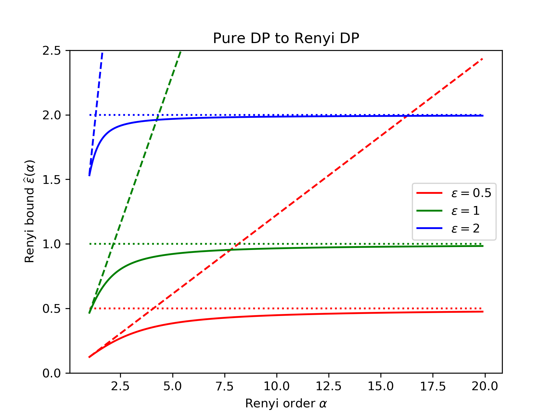This first plot compares the tight Rényi DP bound from Theorem 4 (solid line) with the trivial bound (\(\widehat\varepsilon(\alpha)\le\varepsilon\), dotted line) and the bound implied by zCDP (\(\widehat\varepsilon(\alpha)\le\alpha\rho\), dashed line) via Theorem 5. We consider \(\varepsilon=\frac12\) (red lines, bottom), \(\varepsilon=1\) (green lines, middle), and \(\varepsilon=2\) (blue lines, top).

We see that the trivial bound is tight as the Rényi order \(\alpha\) becomes large, while the zCDP bound is tight for small Rényi orders (i.e., \(\alpha\to1\)). The smaller \(\varepsilon\) is, the later this transition occurs.

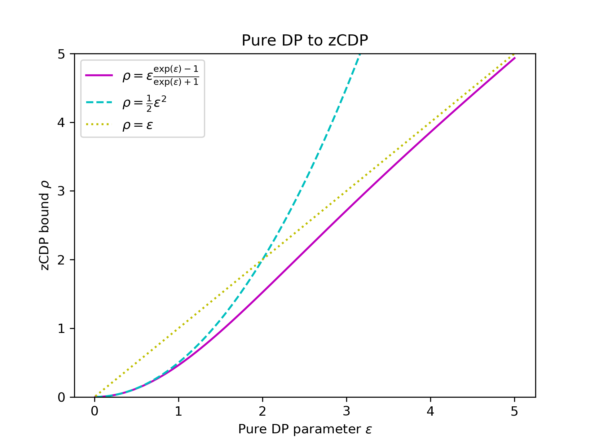
This second plot compares the tight zCDP bound from Theorem 5 (solid magenta line) against the trivial bound (dotted yellow line) and the quadratic bound (dashed cyan line).

We see that, for small values of \(\varepsilon\), the quadratic bound is tight, while for large values of \(\varepsilon\), the trivial bound is tight.

Conclusion

In this post, we have given improved bounds for converting from pure DP to Rényi DP and zCDP. Numerically, these bounds are a modest improvement over the standard bounds.

The bounds are tight when the algorithm corresponds to randomized response. However, in many cases we can prove better bounds for specific algorithms. For example, in a previous post, we proved better zCDP bounds for the exponential mechanism.

Another popular pure DP mechanism is Laplace noise addition. Mironov [M17, Proposition 6] computed a tight Rényi DP bound specifically for the Laplace mechanism: Adding Laplace noise with scale \(1/\varepsilon\) to a sensitivity-1 function guarantees \(\varepsilon\)-DP and also \((\alpha,\widehat\varepsilon_{\text{Lap}}(\alpha))\)-RDP for all \(\alpha>1\) and \[\widehat\varepsilon_{\text{Lap}}(\alpha) = \frac{1}{\alpha-1}\log\left( \frac{\alpha}{2\alpha-1} e^{(\alpha-1)\varepsilon} + \frac{\alpha-1}{2\alpha-1} e^{-\alpha\varepsilon} \right).\]

Acknowledgements

Thanks to Damien Desfontaines for prompting this post. To the best of my knowledge this improved conversion first appeared in a Tweet by Yu-Xiang Wang.

---