The study of differentially private PAC learning runs all the way from its introduction in 2008 [KLNRS08] to a best paper award at the Symposium on Foundations of Computer Science (FOCS) this year [BLM20]. In this post, we’ll recap the history of this line of work, aiming for enough detail for a rough understanding of the results and methods.

Before we get to the “what” and “how” of private PAC learning, it’s worth thinking about the “why”. One motivation for this line of work is that it neatly captures a fundamental question: does privacy in machine learning come at a price? Machine learning is now sufficiently successful and widespread for this question to have real import. But to even start to address this question, we need a formalization of machine learning that allows us to reason about possible trade-offs in a rigorous way. Statistical learning theory, and its computational formalization as PAC learning, provide one such clean and well-studied model. We can therefore use PAC learning as a testbed whose insights we might carry to other less idealized forms of learning.

With this motivation in mind, the rest of this post is structured as follows. The first section covers the basics of the PAC model, and subsequent sections gradually build up a chronology of results. When possible, we give short sketches of the accompanying techniques.

PAC Learning

We’ll start with a brief overview of PAC learning absent any privacy restrictions. Readers familiar with PAC learning can probably skip this section while noting that

1. (the cardinality version of) Occam’s razor is a baseline learner using \(O(\log|\mathcal{H}|)\) samples,

2. VC dimension characterizes non-private PAC learning,

3. we’ll focus on the sample complexity of realizable PAC learning,

4. we’ll usually omit dependencies on accuracy and success probability parameters, and

5. we’ll usually ignore computational efficiency.

For readers needing a refresher on PAC learning, the basic element of the “probably approximately correct” (PAC) framework [Val84] is a hypothesis. Each hypothesis is a function \(h \colon \mathcal{X}\to \{-1,1\}\) mapping examples from some space \(\mathcal{X}\) to binary labels. A collection of hypotheses is a hypothesis class \(\mathcal{H}\), e.g., thresholds (a.k.a. perceptrons), rectangles, conjunctions, and so on. In the realizable setting, a learner receives examples drawn from some unknown distribution and labeled by an unknown \(h^\ast \in \mathcal{H}\). The learner’s goal is to with high probability (“probably”) output a hypothesis that mostly matches the labels of \(h^\ast\) on future examples from the unknown example distribution (“approximately correct”). In the agnostic setting, examples are not necessarily labeled by any \(h \in \mathcal{H}\), and the goal is only to output a hypothesis that approximates the best error of any hypothesis from \(\mathcal{H}\). As mentioned above, we focus on the realizable setting unless otherwise specified. In the proper setting, the learner must output a hypothesis from \(\mathcal{H}\) itself. In the improper setting, this requirement is removed.

In general, we say an algorithm \((\alpha,\beta)\)-PAC learns \(\mathcal{H}\) with sample complexity \(n\) if \(n\) samples are sufficient to with probability at least \(1-\beta\) obtain error at most \(\alpha\) over new examples from the distribution. For the purposes of this post, we generally omit these dependencies on \(\alpha\) and \(\beta\), as they typically vary little or not at all when switching between non-private and private PAC learning.

Fortunately, we always have a simple baseline learner based on empirical risk minimization: given a set of labeled examples, iterate over all hypotheses \(h \in \mathcal{H}\), check how many of the labeled examples each \(h\) mislabels, and output a hypothesis that mislabels the fewest examples. Using this learner, which is sometimes called “Occam’s razor,” \(O(\log|\mathcal{H}|)\) samples suffice to PAC learn \(\mathcal{H}\).

At the same time, \(|\mathcal{H}|\) is a pretty coarse measure of hypothesis class complexity, as it would immediately rule out learning any infinite hypothesis class (of which there are many). Thus, as you might expect, we can do better. We do so using VC dimension. \(\mathsf{VCD}\left(\mathcal{H}\right)\) is the size of the largest possible collection of examples such that, for every labeling of the examples, \(\mathcal{H}\) contains a hypothesis with that labeling. With VC dimension, we can essentially swap \(\log|\mathcal{H}|\) with \(\mathsf{VCD}\left(\mathcal{H}\right)\) in the Occam’s razor bound and PAC learn with \(O(\mathsf{VCD}\left(\mathcal{H}\right))\) samples. In fact, the “Fundamental Theorem of Statistical Learning” says that PAC learnability (realizable or agnostic) is equivalent to finite VC dimension. In this sense, \(\mathsf{VCD}\left(\mathcal{H}\right)\) is a good measure of how hard it is to PAC learn \(\mathcal{H}\). As a motivating example that will re-appear later, note that for the hypothesis class of 1-dimensional thresholds over \(T\) points, \(\log |\mathcal{H}| = \log T\), while \(\mathsf{VCD}\left(\mathcal{H}\right)\) is only 1.

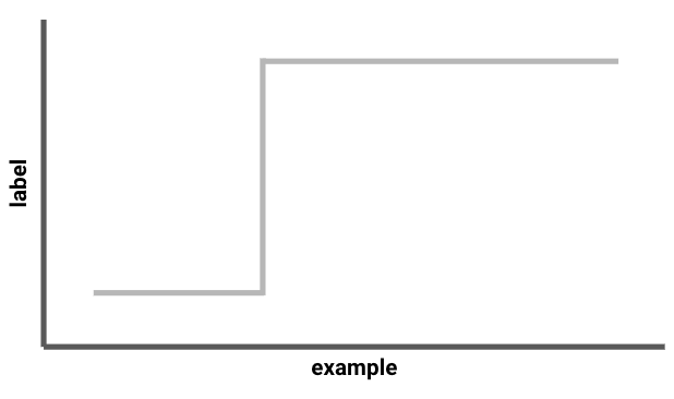An illustration of 1-dimensional thresholds. A given threshold is determined by some point \(x^\ast \in [T]\): any example \(x \leq x^\ast\) receives label \(-1\), and any example \(x > x^\ast\) receives label 1.

A Simple Private PAC Learner

It is straightforward to add a differential privacy constraint to the PAC framework: the hypothesis output by the learner must be a differentially private function of the labeled examples \((x_1, y_1), \ldots, (x_n, y_n)\). That is, changing any one of the examples — even to one with an inconsistent label — must not affect the distribution over hypotheses output by the learner by too much.

Since we haven’t talked about any other PAC learner, we may as well start with the empirical risk minimization-style Occam’s razor discussed in the previous section, which simply selects a hypothesis that minimizes empirical error. A private version becomes easy if we view this algorithm in the right light. All it is doing is assigning a score to each possible output (the hypothesis’ empirical error) and outputting one with the best (lowest) score. This makes it a good candidate for privatization by the exponential mechanism [MT07].

Recall that the exponential mechanism uses a scoring function over outputs to release better outputs with higher probability, subject to the privacy constraint. More formally, the exponential mechanism requires a scoring function \(u(X,h)\) mapping (database, output) pairs to real-valued scores and then selects a given output \(h\) with probability proportional to \(\exp\left(\tfrac{\varepsilon u(X,h)}{2\Delta(u)}\right)\). Thus a lower \(\varepsilon\) (stricter privacy requirement) and larger \(\Delta(u) := \sup_h \sup_{X \sim X’} u(X,h) - u(X’,h) \) (scoring function more sensitive to changing one element in the database \(X\) to make \(X’\)) both lead to a more uniform (more private) output distribution.

Fortunately for our PAC learning setting, empirical error is not a very sensitive scoring function: changing one sample only changes empirical error by 1. We can therefore use (negative) empirical error as our scoring function \(u(X,h)\), apply the exponential mechanism, and get a “private Occam’s razor.” This was exactly what Kasiviswanathan, Lee, Nissim, Raskhodnikova, and Smith [KLNRS08] did when they introduced differentially private PAC learning in 2008. The resulting sample complexity bounds differ from the generic Occam’s razor only by an \(\varepsilon\) factor in the denominator, and \(O(\log|\mathcal{H}|/\varepsilon)\) samples suffice to privately PAC learn \(\mathcal{H}\).

Of course, our experience with non-private PAC learning suggests that we shouldn’t be satisfied with this \(\log |\mathcal{H}|\) dependence. Maybe VC dimension characterizes private PAC learning, too?

Characterizing Pure Private PAC Learning

As it turns out, answering this question will take some time. We start with a partial negative answer. Specifically, we’ll see a class with VC dimension 1 and (a restricted form of) private sample complexity arbitrarily larger than 1. We’ll also cover the first in a line of characterization results for private PAC learning.

We first consider learners that satisfy pure privacy. Recall that pure \((\varepsilon,0)\)-differential privacy forces output distributions that may only differ by a certain \(e^\varepsilon\) multiplicative factor (like the exponential mechanism above). The strictly weaker notion of approximate \((\varepsilon,\delta)\)-differential privacy also allows a small additive \(\delta\) factor. Second, we restrict ourselves to proper learners, which may only output hypotheses from the learned class \(\mathcal{H}\).

With these assumptions in place, in 2010, Beimel, Kasiviswanathan, and Nissim [BKN10] studied a hypothesis class called \(\mathsf{Point}_d\). \(\mathsf{Point}_d\) consists of \(2^d\) hypotheses, one for each vector in \(\{0,1\}^d\). Taking the set of examples \(\mathcal{X}\) to be \(\{0,1\}^d\) as well, we define each hypothesis in \(\mathsf{Point}_d\) to label only its associated vector as 1, and the remaining \(2^d-1\) examples as -1. [BKN10] showed that the hypothesis class \(\mathsf{Point}_d\) requires \(\Omega(d)\) samples for proper pure private PAC learning. In contrast, \(\mathsf{VCD}\left(\mathsf{Point}_d\right) = 1\), so this \(\Omega(d)\) lower bound shows us that VC dimension does not characterize proper pure private PAC learning.

This result uses the classic “packing” lower bound method, which powers many lower bounds for pure differential privacy. The general packing method is to first construct a large collection of databases which are all “close enough” to each other but nonetheless all have different “good” outputs. Once we have such a collection, we use group privacy. Group privacy is a corollary of differential privacy that requires databases differing in \(k\) elements to have \(k\varepsilon\)-close output distributions. Because of group privacy, if we start with a collection of databases that are close together, then the output distributions for any two databases in the collection cannot be too different. This creates a tension: utility forces the algorithm to produce different output distributions for different databases, but privacy forces similarity. The packing argument comes down to arguing that, unless the databases are large, privacy wins out, and when privacy wins out then there is some database where the algorithm probably produces a bad output.

For \(\mathsf{Point}_d\), we sketch the resulting argument as follows. Suppose we have an \(\varepsilon\)-private PAC learner that uses \(m\) samples. Then we can define a collection of different databases of size \(m\), one for each hypothesis in \(\mathsf{Point}_d\). By group privacy, the output distribution for our private PAC learner changes by at most \(e^{m\varepsilon}\) between any two of the databases in this collection. Thus we can pick any \(h \in \mathsf{Point}_d\) and know that the probability of outputting the wrong hypothesis is at least roughly \(2^d \cdot e^{-m\varepsilon}\). Since we need this probability to be small, rearranging implies \(m = \Omega(d/\varepsilon)\).

[BKN10] then contrasted this result with an improper pure private PAC learner. This learner applies the exponential mechanism to a class \(\mathsf{Point}_d’\) of hypotheses derived from \(\mathsf{Point}_d\) — but not necessarily a subset of \(\mathsf{Point}_d\) — gives an improper pure private PAC learner with sample complexity \(O(\log d)\). Since this learner is improper, it circumvents the “one database per hypothesis” step of the packing lower bound. Moreover, [BKN10] gave a still more involved improper pure private PAC learner requiring only \(O(1)\) samples. This separates proper pure private PAC learning from improper pure private PAC learning. In contrast, the sample complexities of proper and improper PAC learning absent privacy are the same up to logarithmic factors in \(\alpha\) and \(\beta\).

In 2013, Beimel, Nissim, and Stemmer [BNS13] proved a more general result. They gave the first characterization of pure (improper) private PAC learning by defining a new hypothesis class measure called the representation dimension, \(\mathsf{REPD}\left(\mathcal{H}\right)\). Roughly, the representation dimension considers the collection of all distributions \(\mathcal{D}\) over sets of hypotheses, not necessarily from \(\mathcal{H}\), that “cover” \(\mathcal{H}\). By “cover,” we mean that for any \(h \in \mathcal{H}\), with high probability a set drawn from covering distribution \(\mathcal{D}\) includes a hypothesis that mostly produces labels that agree with \(h\). With this collection of distributions defined, \(\mathsf{REPD}\left(\mathcal{H}\right)\) is the minimum over all such covering distributions of the logarithm of the size of the largest set in its support. Thus a hypothesis class that can be covered by a distribution over small sets of hypotheses will have a small representation dimension. With the notion of representation dimension in hand, [BNS13] gave the following result:

Theorem 1 ([BNS13]). The sample complexity to pure private PAC learn \(\mathcal{H}\) is \(\Theta(\mathsf{REPD}\left(\mathcal{H}\right))\).

Representation dimension may seem like a strange definition, but a sketch of the proof of this result helps illustrate the connection to private learning. Recall from our private Occam’s razor, and the improper pure private PAC learner above, that if we can find a good and relatively small set of hypotheses to choose from, then we can apply the exponential mechanism and call it a day. It is exactly this kind of “good set of hypotheses” that representation dimension aims to capture. A little more formally, given an upper bound on \(\mathsf{REPD}\left(\mathcal{H}\right)\), we know there is some covering distribution whose largest hypothesis set is not too big. That means we can construct a learner that draws a hypothesis set from this covering distribution and applies the exponential mechanism to it. Just as we picked up a \(\log|\mathcal{H}|\) sample complexity dependence using private Occam’s razor, since \(\mathsf{REPD}\left(\mathcal{H}\right)\) measures the logarithm of the size of the largest hypothesis set in the support, this pure private learner picks up a \(\mathsf{REPD}\left(\mathcal{H}\right)\) sample complexity dependence here. This gives us one direction of Theorem 1.

This logic works in the other direction as well. To go from a pure private PAC learner with sample complexity \(m\) to an upper bound on \(\mathsf{REPD}\left(\mathcal{H}\right)\), we return to the group privacy trick used by [BKN10]. Suppose we fix a database of size \(m\) and pass it to the learner. By group privacy and the learner’s accuracy guarantee, if we fix some concept \(c\), the learner has probability at least roughly \(e^{-m}\) of outputting a hypothesis that mostly agrees with \(c\). Thus if we repeat this process roughly \(e^{m}\) times, we probably get at least one hypothesis that mostly agrees with \(c\). In other words, this repeated calling of the learner on the arbitrary database yields a covering distribution for \(\mathcal{H}\). Since we called the learner approximately \(e^m\) times, the logarithm of this is \(m\), and we get our upper bound on \(\mathsf{REPD}\left(\mathcal{H}\right)\).

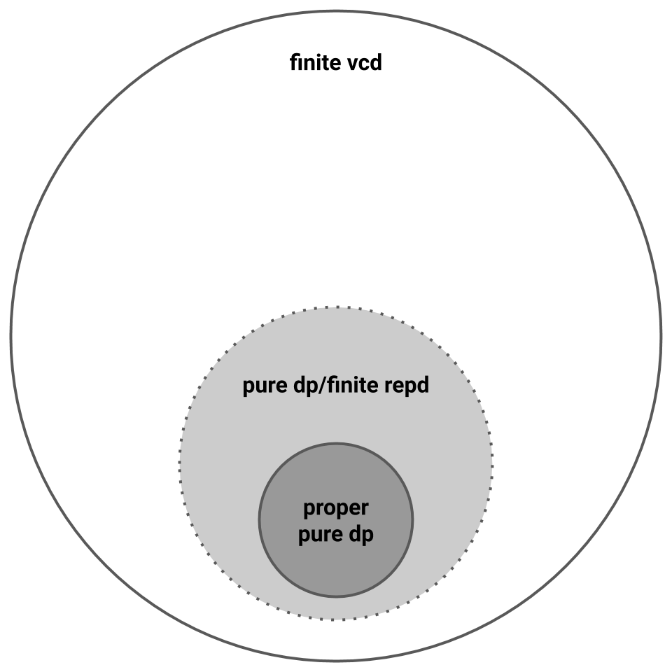
To recap, we now know that proper pure private PAC learning is strictly harder than improper pure private PAC learning, which is characterized by representation dimension. A picture sums it up. Note the dotted line, since we don’t yet have any evidence separating finite representation dimension and finite VC dimension.

Separating Pure and Approximate Private PAC Learning

So far, we’ve focused only on pure privacy. In this section, we move on to the first separations between pure and approximate private PAC learning, as well as the first connection between private learning and online learning.

Our source is a pair of interconnected papers from around 2014. Among other things, Feldman and Xiao [FX14] introduced Littlestone dimension to private PAC learning. By connecting representation dimension to results from communication complexity to Littlestone dimension, they proved the following:

Theorem 2 ([FX14]). The sample complexity to pure private PAC learn \(\mathcal{H}\) is \(\Omega(\mathsf{LD}\left(\mathcal{H}\right))\).

Littlestone dimension \(\mathsf{LD}\left(\mathcal{H}\right)\) is, roughly, the maximum number of mistakes an adversary can force an online PAC-learning algorithm to make [Lit88]. We always have \(\mathsf{VCD}\left(\mathcal{H}\right) \leq \mathsf{LD}\left(\mathcal{H}\right) \leq \log|\mathcal{H}|\), but these inequalities can be strict. For example, denoting by \(\mathsf{Thresh_T}\) the class of thresholds over \(\{1, 2, \ldots, T\}\), since an adversary can force \(\Theta(\log T)\) wrong answers from an online learner binary searching over \(\{1,2, \ldots, T\}\), \(\mathsf{LD}\left(\mathsf{Thresh_T}\right) = \Omega(\log T)\). In contrast, \(\mathsf{VCD}\left(\mathsf{Thresh_T}\right) = 1\).

At first glance it’s not obvious what Theorem 2 adds over Theorem 1. After all, Theorem 1 gives an equivalence, not just a lower bound. One advantage of Theorem 2 is that Littlestone dimension is a known quantity that has already been studied in its own right. We can now import results like the lower bound on \(\mathsf{LD}\left(\mathsf{Thresh_T}\right)\), whereas bounds on \(\mathsf{REPD}\left(\cdot\right)\) are not common. A second advantage is that Littlestone dimension conceptually connects private learning and online learning: we now know that pure private PAC learning is no easier than online PAC learning.

A second paper by Beimel, Nissim, and Stemmer [BNS13b] contrasted this \(\Omega(\log T)\) lower bound for pure private learning of thresholds with a \(2^{O(\log^\ast T)}\) upper bound for approximate private PAC learning \(\mathsf{Thresh_T}\). Here \(\log^\ast\) denotes the very slow-growing iterated logarithm, the number of times we must take the logarithm of the argument to bring it \(\leq 1\). (We’re not kidding about “very slow-growing” either: \(\log^\ast(\text{number of atoms in universe}) \approx 4\).) With Feldman and Xiao’s result, this separates pure private PAC learning from approximate private PAC learning. It also shows that representation dimension does not characterize approximate private PAC learning.

At the same time, Feldman and Xiao observed that the connection between pure private PAC learning and Littlestone dimension is imperfect. Again borrowing results from communication complexity, they observed that the hypothesis class \(\mathsf{Line_p}\) (which we won’t define here) has \(\mathsf{LD}\left(\mathsf{Line_p}\right) = 2\) but \(\mathsf{REPD}\left(\mathsf{Line_p}\right) = \Theta(\log(p))\). In contrast, they showed that an approximate private PAC learner can learn \(\mathsf{Line_p}\) using \(O\left(\tfrac{\log(1/\beta)}{\alpha}\right)\) samples. Since this entails no dependence on \(p\) at all, it improves the separation between pure and approximate private PAC learning given by [BNS13b].

Let’s pause to recap what’s happened so far. We learned in the last section that representation dimension characterizes pure private PAC learning [BNS13]. We learned in this section that Littlestone dimension gives lower bounds for pure private PAC learning but, as shown by \(\mathsf{Line_p}\), these bounds are sometimes quite loose [FX14]. \(\mathsf{Thresh_T}\) shows that representation dimension does not characterize approximate private PAC learning [FX14 ; BNS13b], and we still have no privacy-specific lower bounds for approximate private learners. So the picture now looks like this:

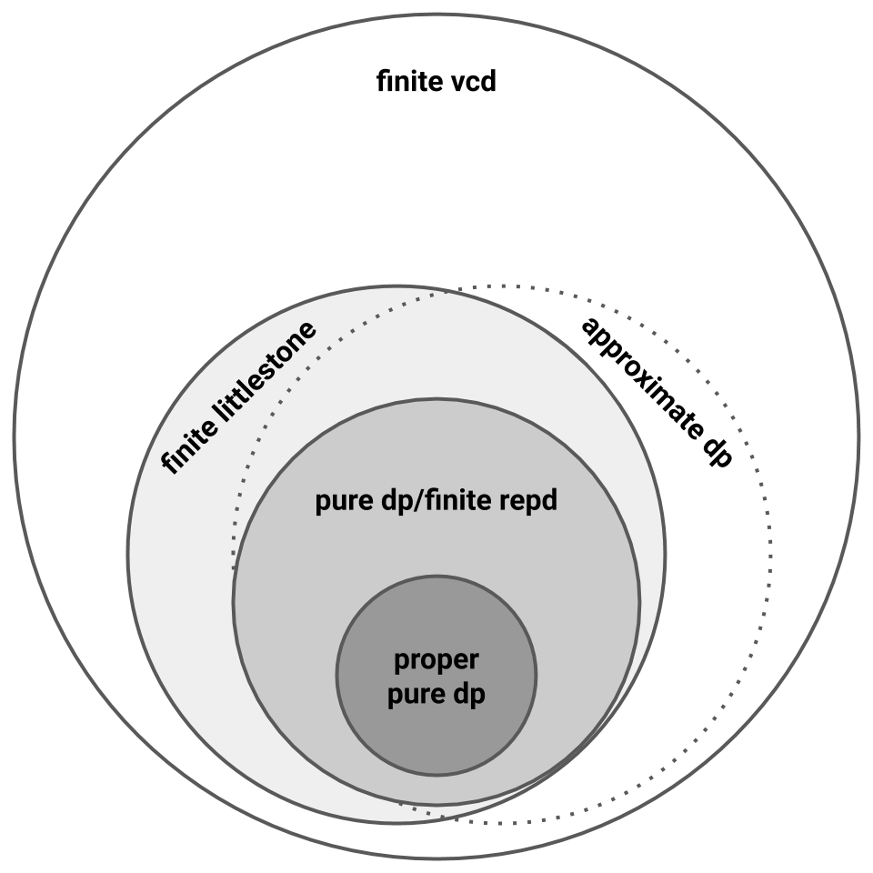
In particular, we might still find that VC dimension characterizes approximate private PAC learning!

Lower Bounds for Approximate Private PAC Learning

We now dash this hope. In 2015, Bun, Nissim, Stemmer, and Vadhan [BNSV15] gave the first nontrivial lower bound for approximate private PAC learning. They showed that learning \(\mathsf{Thresh_T}\) has proper approximate private sample complexity \(\Omega(\log^\ast(T))\) and \(O(2^{\log^\ast(T)})\).

We’ll at least try to give some intuition for the presence of \(\log^\ast\) in the lower bound. Informally, the lower bound relies on an inductive construction of a sequence of hard problems for databases of size \(n=1, 2, \ldots\). The \(k^{th}\) hard problem relies on a distribution over databases of size \(k\) whose data universe is of of size exponential in the size of the data universe for the \((k-1)^{th}\) distribution. The base case is the uniform distribution over the two singleton databases \(\{0\}\) and \(\{1\}\), and they show how to inductively construct successive problems such that a solution for the \(k^{th}\) problem implies a solution for the \((k-1)^{th}\) problem. Unraveling the recursive relationship between the problem domain sizes implies a general lower bound of roughly \(\log^\ast|X|\) for domain \(X\).

The inclusion of \(\log^\ast\) makes this is an extremely mild lower bound. However, \(\log^\ast(T)\) can still be arbitrarily larger than 1, so this is the first definitive evidence that proper approximate privacy introduces a cost over non-private PAC learning.

In 2018, Alon, Livni, Malliaris, and Moran [ALMM19] extended this \(\Omega(\log^\ast T)\) lower bound for \(\mathsf{Thresh_T}\) to improper approximate privacy. More generally, they gave concrete evidence for the importance of thresholds, which have played a seemingly outsize role in the work so far. They did so by relating a class’ Littlestone dimension to its ability to “contain” thresholds. Here, we say \(\mathcal{H}\) “contains” \(m\) thresholds if there exist \(m\) (unlabeled) examples \(x_1,\ldots,x_m\) and hypotheses \(h_1, \ldots, h_m \in \mathcal{H}\) such that the hypotheses “behave like” thresholds on the \(m\) examples, i.e., \(h_i(x_j) = 1 \Leftrightarrow j \geq i\). With this language, they imported a result from model theory to show that any hypothesis class \(\mathcal{H}\) contains \(\log(\mathsf{LD}\left(\mathcal{H}\right))\) thresholds. This implies that learning \(\mathcal{H}\) is at least as hard as learning \(\mathsf{Thresh_T}\) with \(T = \log(\mathsf{LD}\left(\mathcal{H}\right))\). Since \(\log^\ast(\log(\mathsf{LD}\left(\mathcal{H}\right))) = \Omega(\log^\ast(\mathsf{LD}\left(\mathcal{H}\right)))\), combining these two results puts the following limit on private PAC learning:

Theorem 3 ([ALMM19]). The sample complexity to approximate private PAC learn \(\mathcal{H}\) is \(\Omega(\log^\ast(\mathsf{LD}\left(\mathcal{H}\right)))\).

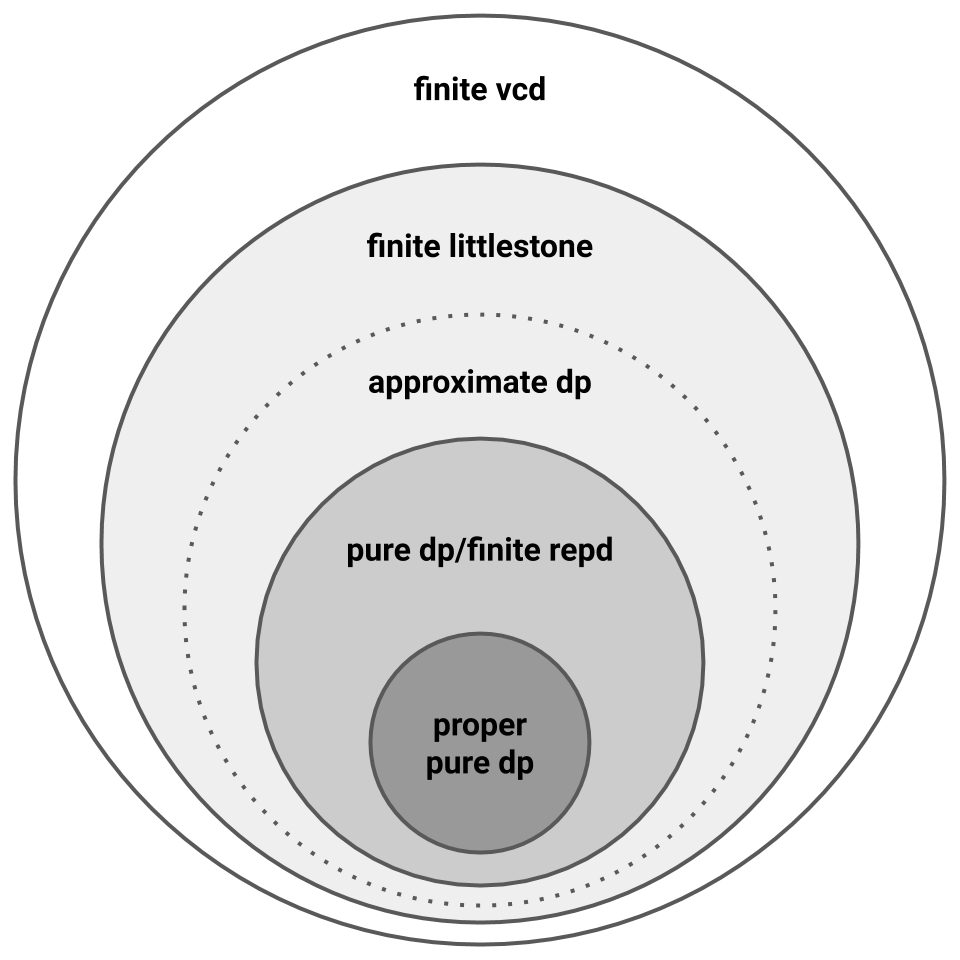
Littlestone dimension characterizes online PAC learning, so we now know that online PAC learnability is necessary for private PAC learnability. Sufficiency, however, remains an open question. This produces the following picture, where the dotted line captures the question of sufficiency.

Characterizing Approximate Private PAC Learning

Spurred by this question, several advances in private PAC learning have appeared in the last year. First, Gonen, Hazan, and Moran strengthened Theorem 3 by giving a constructive method for converting pure private learners to online learners [GHM19]. Their result reaches back to the 2013 characterization of pure private learning in terms of representation dimension by using the covering distribution to generate a collection of “experts” for online learning. Again revisiting \(\mathsf{Thresh_T}\), Kaplan, Ligett, Mansour, Naor, and Stemmer [KLMNS20] significantly reduced the \(O(2^{\log^\ast(T)})\) upper bound of [BNSV15] to just \(O((\log^\ast(T))^{1.5})\). And Alon, Beimel, Moran, and Stemmer [ABMS20] justified this post’s focus on realizable private PAC learning by giving a transformation from a realizable approximate private PAC learner to an agnostic one at the cost of slightly worse privacy and sample complexity. This built on an earlier transformation that only applied to proper learners [BNS15].

Finally, Bun, Livni, and Moran [BLM20] answered the open question posed by [ALMM19]:

Theorem 4 ([BLM20]). The sample complexity to approximate private PAC learn \(\mathcal{H}\) is \(2^{O({\mathsf{LD}\left(\mathcal{H}\right)})}\).

To prove this, [BLM20] introduced the notion of a globally stable learner and showed how to convert an online learner to a globally stable learner to a private learner. Thus, combined with the result of [ALMM19], we now know that the sample complexity of private PAC learning any \(\mathcal{H}\) is at least \(\Omega(\log^\ast(\mathsf{LD}\left(\mathcal{H}\right)))\) and at most \(2^{O({\mathsf{LD}\left(\mathcal{H}\right)})}\). In this sense, online learnability characterizes private learnability.

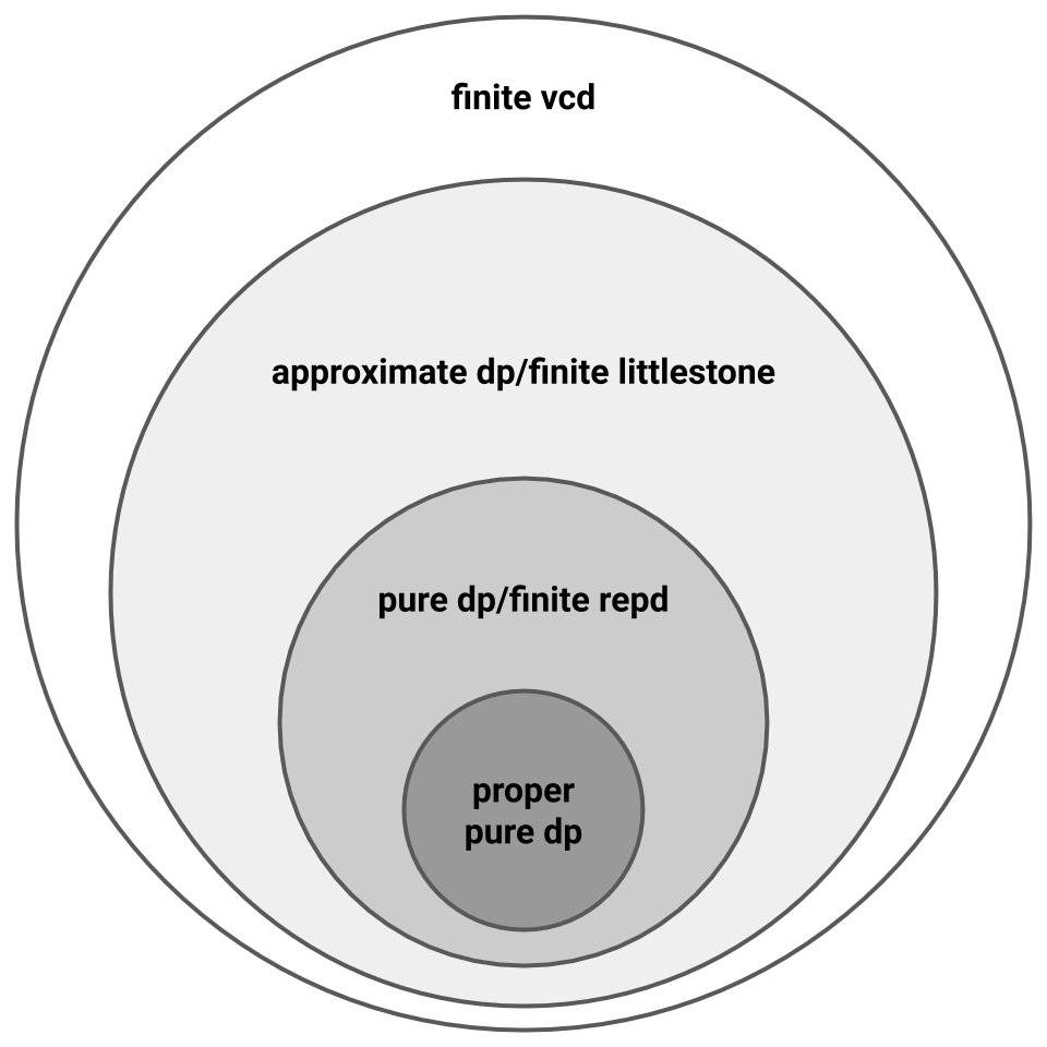
Narrowing the gap between the lower and upper bounds above is an open question. Note that we cannot hope to close the gap completely. For the lower bound, the current \(\mathsf{Thresh_T}\) upper bound implies that no general lower bound can be stronger than \(\Omega((\log^\ast(\mathsf{LD}\left(\mathcal{H}\right)))^{1.5})\). For the upper bound, there exist hypotheses classes \(\mathcal{H}\) with \(\mathsf{VCD}\left(\mathcal{H}\right) = \mathsf{LD}\left(\mathcal{H}\right)\) (e.g., \(\mathsf{VCD}\left(\mathsf{Point}_d\right) = \mathsf{LD}\left(\mathsf{Point}_d\right)= 1\)), so since non-private PAC learning requires \(\Omega(\mathsf{VCD}\left(\mathcal{H}\right))\) samples, the best possible private PAC learning upper bound is \(O(\mathsf{LD}\left(\mathcal{H}\right))\). Nevertheless, proving either bound remains open.

Conclusion

This concludes our post, and with it our discussion of this fundamental question: the price of privacy in machine learning. We now know that in the PAC model, proper pure private learning, improper pure private learning, approximate private learning, and non-private learning are all strongly separated. By the connection to Littlestone dimension, we also know that approximate private learnability is equivalent to online learnability. However, many questions about computational efficiency and tight sample complexity bounds remain open.

As mentioned in the introduction, we focused on the clean yet widely studied and influential model of PAC learning. Having characterized how privacy enters the picture in PAC learning, we can hopefully convey this understanding to other models of learning, and now approach these questions from a rigorous and grounded point of view.

Congratulations to Mark Bun, Roi Livni, and Shay Moran on their best paper award — and to the many individuals who paved the way before them!

Acknowledgments

Thanks to Kareem Amin and Clément Canonne for helpful feedback while writing this post.