Limits of Privacy Amplification by Subsampling
In our previous post we gave a brief introduction to privacy amplification by subsampling. The high-level story is that we can make differentially private algorithms faster by runninng them on a subsample of the dataset instead of the whole dataset and this comes at essentially no cost in privacy and accuracy. That story is pretty good. But now we’ll take a closer look at the details of this story.
Setting
Recall that we’re comparing the standard Laplace mechanism \(M(x) := \frac{1}{n}\sum_{x_i \in x} q(x_i) + \mathsf{Laplace}\left(\frac{1}{\varepsilon n}\right)\) to the subsampled Laplace mechanism \(\widetilde{M}_{p}(x) := \frac{1}{pn} \sum_{x_i \in S_p(x)} q(x_i) + \mathsf{Laplace}\left(\frac{1}{\varepsilon_p p n}\right)\), where \(S_p(x)\subseteq x\) is a random Poisson subsample that includes each person’s data independently with probability \(p\). Both algorithms satisfy the same \(\varepsilon\)-differential privacy guarantee. The respective mean squared error guarantees are \[\mathbb{E}\left[\left(M(x) - \frac{1}{n}\sum_{x_i \in x} q(x_i)\right)^2\right] = \frac{2}{\varepsilon^2 n^2}. \tag{1}\] and \[ \mathbb{E}\left[\left(\widetilde{M}_p(x) - \frac{1}{n}\sum_{x_i \in x} q(x_i) \right)^2\right] \le \frac{|x|}{p n^2} + \frac{2}{\varepsilon_p^2 p^2 n^2} \approx \frac{1}{p n} + \frac{2}{\varepsilon^2 n^2},\tag{2}\] where \[\varepsilon_p = \log\left(1 + \frac{1}{p} \big( e^{\varepsilon}-1 \big)\right) \approx \frac{\varepsilon}{p}. \tag{3} \]
Comparing Equation 1 with Equation 2, there are two differences: The non-private statistical error \(\frac{1}{p n}\) and the approximation from Equation 3. We’ll ignore the non-private statistical error \(\frac{1}{p n}\) in this post, since it isn’t the dominant error term for reasonable parameter regimes and, well, this is DifferentialPrivacy.org not Statistics.org.
How good is the approximation?
So let’s talk about the approximation in Equation 3, which directly affects the scale of the Laplace noise added by the subsampled mechanism \(\widetilde{M}_p\): \[\text{noise_scale}(\widetilde{M}_p) = \frac{1}{\varepsilon_p p n} = \frac{1}{pn\log\left(1 + \frac{1}{p} \big( e^{\varepsilon}-1 \big)\right)} \approx \frac{1}{\varepsilon n} = \text{noise_scale}(M). \tag{4} \] The approximation in Equation 3 comes from the Taylor series around \(\varepsilon=0\): \[\varepsilon_p = \log\left(1 + \frac{1}{p} \big( e^{\varepsilon}-1 \big)\right) = \frac{\varepsilon}{p} - \frac{(1-p)\varepsilon^2}{2p^2} + \frac{(2-p)(1-p)\varepsilon^3}{6p^3} \pm O(\varepsilon^4)\tag{5}.\] The approximation in Equation 3 is just the first term in this Taylor series.1 We can make the approximation precise with some inequalities:2 \[\frac{\varepsilon}{p+\varepsilon} \le \log\left(1 + \frac{\varepsilon}{p}\right) \le \varepsilon_p = \log\left(1 + \frac{1}{p} \big( e^{\varepsilon}-1 \big)\right) \le \frac{\varepsilon}{p}. \tag{6} \]
To get an idea of how good this approximation actually is, let’s plot the approximation ratio \[\frac{\text{noise_scale}(M)}{\text{noise_scale}(\widetilde{M}_p)} = \frac{p\varepsilon_p}{\varepsilon} = \frac{p}{\varepsilon} \log\left(1 + \frac{1}{p} \big( e^{\varepsilon}-1 \big)\right) \approx 1:\tag{7}\] (Per Equation 6, this ratio is bounded: \(\frac{p}{p+\varepsilon} \le \frac{p\varepsilon_p}{\varepsilon} \le 1\).)
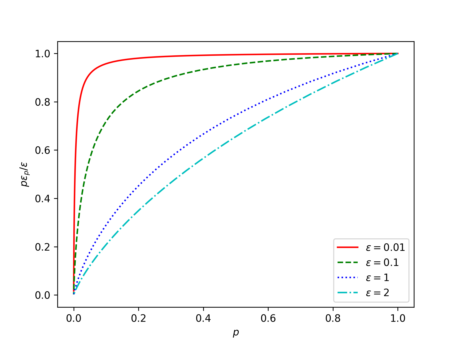

This doesn’t look so good! The approximation we made in Equation 3 tells us that all of the plotted lines should be close to 1. But this seems to only be accurate when the subsampling probability \(p\) is large or when the privacy parameter \(\varepsilon\) is very small. Large subsampling probability \(p\) doesn’t make much sense for subsampling; we don’t get much speedup. So the question is how small does the privacy parameter \(\varepsilon\) need to be?
Roughly, if we want the approximation in Equation 3 to be good within constant factors, then the privacy parameter \(\varepsilon\) needs to scale linearly with the subsampling probability \(p\). I.e., \(\varepsilon=cp\) for a constant \(c\). Let’s see what the ratio looks like for various constants:
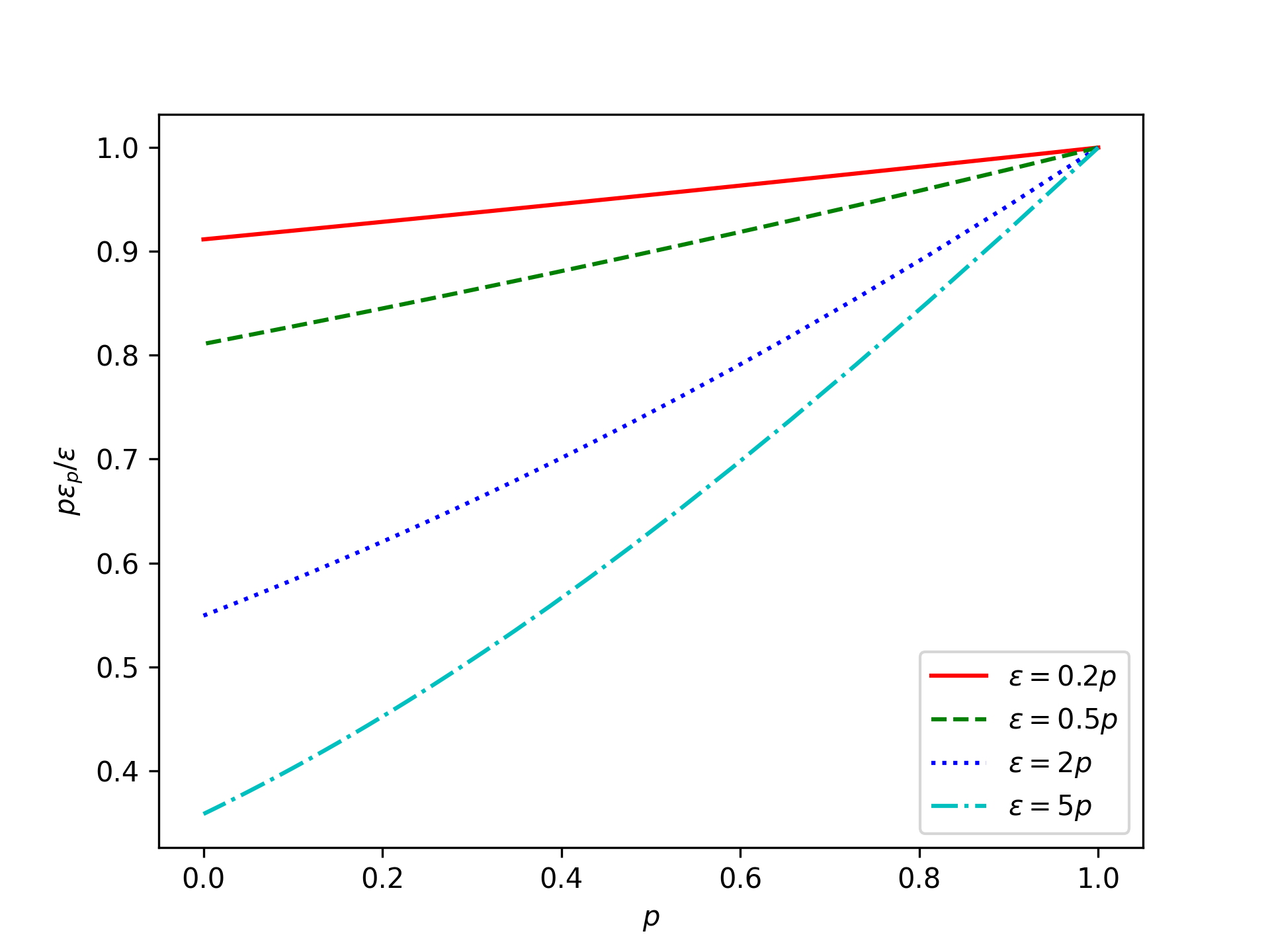
This looks slightly better. In particular, if \(\varepsilon \le 2p\), then \(\frac{p\varepsilon_p}{\varepsilon} \ge \frac{1}{2}\), which means the subsampled Laplace mechanism \(\widetilde{M}_p\) adds at most twice as much noise as the standard Laplace mechanism \(M\).
In general, if we set \(\varepsilon \le cp\), then the ratio in Equation 7 is lower bounded by \[\inf_{p\in(0,1],\varepsilon \in (0,cp]}\frac{p}{\varepsilon} \log\left(1 + \frac{1}{p} \big( e^{\varepsilon}-1 \big)\right) = \frac{1}{c} \log\big( 1+c\big).\tag{8}\] In other words, if \(\varepsilon \le cp\), then the subsampled Laplace mechanism \(\widetilde{M}_p\) adds at most \(\frac{c}{\log(1+c)}\) times as much noise as the standard Laplace mechanism \(M\). Here’s what this function looks like:
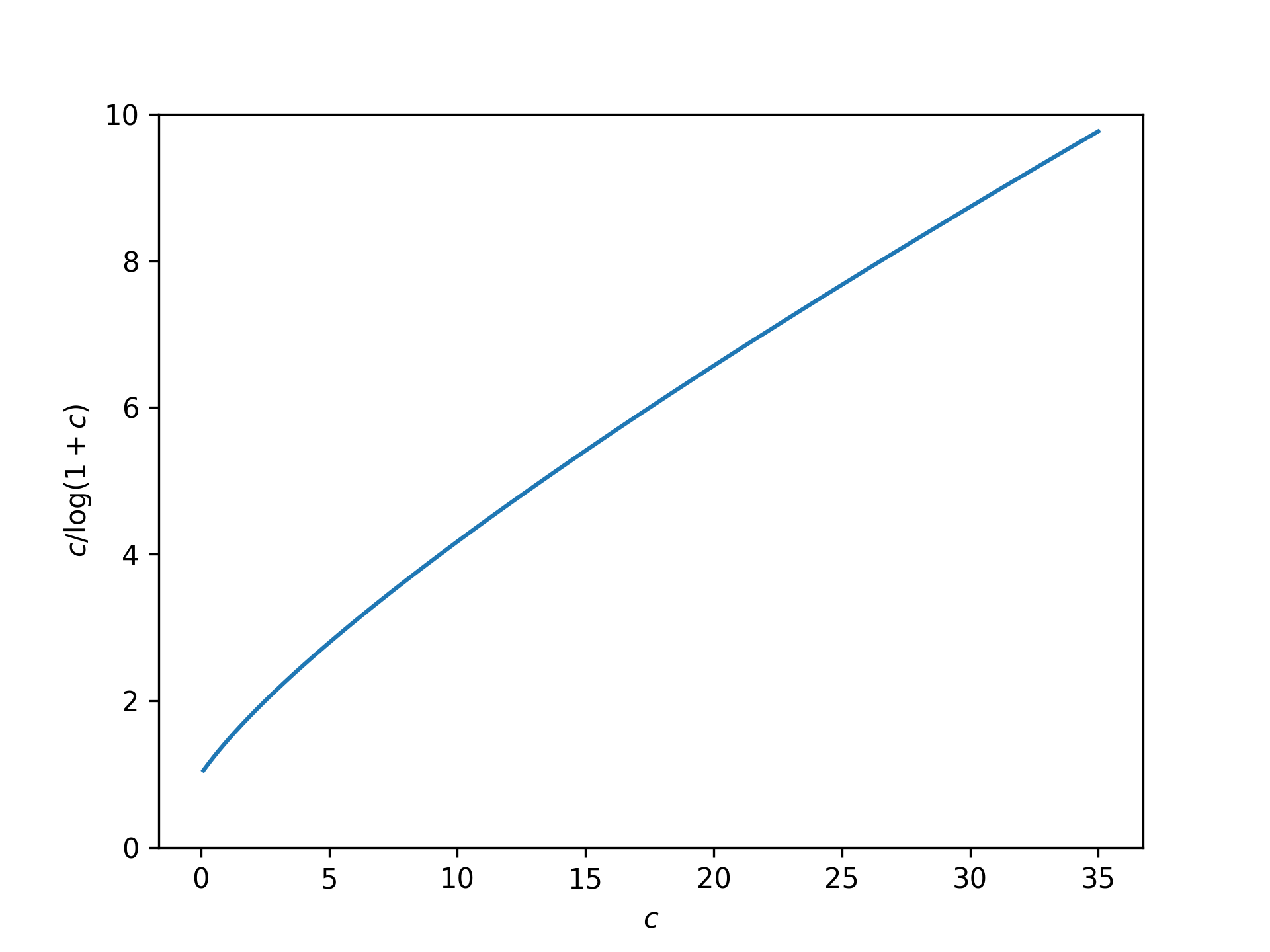
This bound on the ratio seems reasonable as long as \(c\) isn’t large. However, assuming \(\varepsilon \le cp\) is a pretty strong assumption! This is the big limitation of privacy amplification by subsampling – subsampling is free only when the privacy parameter is tiny.
Is \(\varepsilon \le c p \) a reasonable parameter regime?
It depends…
Let’s think about the machine learning application that is the biggest motivation for studying privacy amplification by subsampling.
In machine learning applications we want to answer many queries \(q_1,q_2,\cdots,q_k\). (These queries are actually high-dimensional gradients that we want to estimate, but that’s not important right now.) Suppose we have some overall privacy budget \(\varepsilon_*\). Then this needs to be divided among the \(k\) queries. Using advanced composition, we get a per-query budget of \(\varepsilon = \Theta\left(\frac{\varepsilon_*}{\sqrt{k}}\right)\).3
The overall privacy budget \(\varepsilon_*\) is a constant. So as the number of queries \(k\) increases, the per-query privacy budget shrinks; \(\varepsilon = \Theta(1/\sqrt{k})\). That’s good for subsampling; we are in the small \(\varepsilon\) regime.
Now we want \(\varepsilon \le cp\) for privacy amplification by subsampling, where \(c\) is a small constant. Thus we need \(p \ge \Omega(1/\sqrt{k})\) in the machine learning application. Is this reasonable?
The quantity \(pk\) is the expected number of times each datapoint will be sampled over the \(k\) queries. In machine learning parlance, \(pk\) is the number of training epochs and \(k\) is the number of steps. Thus \(p \ge \Omega(1/\sqrt{k})\) implies that the number of epochs is \(pk \ge \Omega(\sqrt{k})\), which is a lot. It’s common to train with as little as one epoch.
The expected size of each subsample (a.k.a. the batch size) is \(p|x|\), where \(|x|\) is the overall dataset size. We typically want the batch size to be a moderate constant – e.g., 32.4 So we want \(p \le O(1/|x|)\), but privacy amplification by subsampling would need us to set \(\varepsilon \le cp \le O(1/|x|)\). As before, with \(\varepsilon = \Theta(1/\sqrt{k})\), this would correspond to \(k \ge \Omega(|x|^2)\) steps and \(kp \ge \Omega(|x|)\) epochs. The number of steps being quadratic in the dataset size and the number of epochs being linear in the datset size is a lot.
The takeaway from this back-of-the-envelope calculation is that \(\varepsilon \le cp\) is well outside the typical parameter regime for machine learning applications. We have to set the hyperparameters differently for private machine learning.
Conclusion
To summarize, in our previous post the story was that privacy amplification by subsampling can be used to make differentially private algorithms faster and this comes at essentially no cost in privacy and accuracy. But, in this post, we observe that this is free only if the privacy parameter \(\varepsilon\) is tiny. Specifically, the privacy parameter needs to be on the order of the subsampling probability – i.e., \(\varepsilon\le O(p)\) – for the claim to hold up to constant factors.
In these posts, we’ve looked at univariate queries with Laplace noise. In the machine learning application, we would instead have high-dimensional queries (i.e., model gradients) with Gaussian noise. This adds a fair bit of complexity, but the moral of the story remains the same.5
Practitioners of differentially private machine learning have observed that larger batch sizes yield better results. The purpose of this post is to make this folklore knowledge more widely accessible.
To be clear, the limits of privacy amplification by subsampling are a very real problem in practice. Increasing the batch size mitigates the problem, but often comes at a high computational cost.4 Thus, in recent years, there has been a lot of research that seeks to avoid the limits of privacy amplification by subsampling.6
-
Looking at the second- and third-order terms in the Taylor series in Equation 5, we can already see that this approximation may be problematic when the subsampling probability \(p\) is small, since these terms include factors of \(1/p^2\) and \(1/p^3\) respectively. ↩
-
To prove the inequalities in Equation 6: Since \(\log\) is concave, Jensen’s inequality gives \(\log(1-p+pe^{\varepsilon/p}) \ge (1-p)\log(1) + p \log(e^{\varepsilon/p}) = \varepsilon\); rearranging yields the upper bound \(\varepsilon/p \ge \log(1+(e^\varepsilon-1)/p)\). On the other hand \(\varepsilon \le e^\varepsilon-1\), which yields the first inequality on the lower bound side. Finally, we have \(\log(1+x) = \int_0^x \frac{1}{1+t} \mathrm{d}t \ge \int_0^x \frac{1}{(1+t)^2} \mathrm{d}t = \frac{x}{1+x}\) for all \(x\ge0\); substituting \(x=\varepsilon/p\) yields the second inequality on the lower bound side. ↩
-
We’re being a bit imprecise here. We can’t apply advanced composition with pure \((\varepsilon,0)\)-differential privacy. So the overall privacy budget \(\varepsilon_*\) needs to be quantified in terms of approximate \((\varepsilon_*,\delta_*)\)-differential privacy, concentrated differential privacy, or something like that. To make things formal we could set the overall privacy budget constraint as \(\frac{1}{2}\varepsilon_*^2\)-zCDP, which gives a per-query budget of pure \((\varepsilon=\frac{\varepsilon_*}{\sqrt{k}},0)\)-differential privacy. ↩
-
The ideal batch size (in non-private machine learning) is determined by many factors – ultimately, you try a few settings and use whatever works best. Some very rough intuition: A major factor in determining the right batch size is hardware parallelism/pipelining (and memory constraints). Absent parallelism, smaller batch size is typically better – right down to batch size 1; generally, you make faster progress by updating the model parameters after each gradient computation. However, batch size 1 doesn’t exploit the fact that the computer hardware can usually compute multiple gradients at the same time. Larger batch sizes allow you to get more work out of the hardware in the same amount of time. But once you saturate the hardware, there’s little benefit (non-privately) to larger batch sizes. ↩ ↩2
-
The main added complexity of working with Gaussian noise and high-dimensional queries comes from the fact that we can’t use pure \((\varepsilon,0)\)-differential privacy for the analysis. And, if we use approximate \((\varepsilon,\delta)\)-differential privacy for the analysis, we incur superfluous \(\sqrt{\log(1/\delta)}\) factors. To get a sharper analysis we need to work with Rényi differential privacy or numerically compute the privacy loss distribution. There is a lot of very interesting work on this topic, but the high-level conclusion remains the same. ↩
-
For example, DP-FTRL adds negatively correlated noise instead of independent noise to the queries/gradients. Since DP-FTRL doesn’t rely on privacy amplification by subsampling, the noise added to each query/gradient needs to be large. Instead DP-FTRL relies on the fact that, when you sum up the noisy values, the noise can be made to partially cancel out. In practice, DP-FTRL often works better than relying on privacy amplification by subsampling. Another example alternative is to avoid privacy amplification by subsampling by computing gradients on the full dataset and instead accelerating the computation using second-order methods so that we require fewer iterations. ↩
[cite this]