A simple recipe for private synthetic data generation
In the last blog post, we covered the potential pitfalls of synthetic data without formal privacy guarantees, and motivated the need for differentially private synthetic data mechanisms. In this blog post, we will describe the select-measure-generate paradigm, which is a simple and effective template for designing synthetic data mechanisms. The three steps underlying the select-measure-generate paradigm are illustrated and explained below.
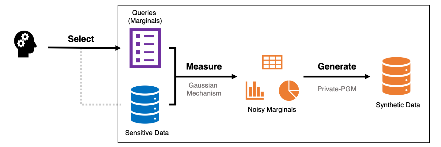
- Select a collection of queries to measure — typically low-dimensional marginals.
- Measure the selected queries privately using a noise-addition mechanism.
- Generate synthetic data that best explains the noisy measurements.1
Mechanisms in this class differ primarily in their methodology for selecting queries and their algorithm for generating synthetic data from noisy measurements. The focus of this blog post is the final Generate step. Specifically, we will explore different ways in which one can model data distributions for the purpose of generating synthetic data, outlining the qualitative pros and cons of each method. We will then introduce the Marginal-Based Inference (MBI) repository that provides methods that, given some set of noisy measurements, enables users to generate synthetic data in a generic and scalable way.
Separating the Generate subroutine from the existing synthetic data generation mechanisms greatly simplifies the design space of new differentially private mechanisms. It allows the mechanism designer to focus on selecting the queries to maximize utility of the synthetic data, rather than how to generate synthetic data that explain the noisy measurements well. Both are challenging technical problems that require different techniques to solve, and MBI provides principled solutions to the latter problem, while exposing an interface that can be readily adopted by mechanism designers.
The Generate Subproblem: A Unifying View
In this section we will introduce the main optimization problem that underlies several methods for the Generate subproblem, and provide a high-level overview of how each method attempts to solve this optimization problem. Let \( y = \mathcal{M}(D) \) be the noisy measurements obtained from running a privacy mechanism on a discrete dataset \( D \). Our goal is to post-process these noise measurements to obtain synthetic data that explains them well. In particular, we wish to minimize over the space of all datasets for one that maximizes the likelihood of the observations \( y \).2
\[ \hat{D} \in \text{arg} \max_{D \in \mathcal{D}} \log \mathbb{P}[\mathcal{M}(D) = y] \]
This is a high-dimensional discrete optimization problem, and is generally intractable to solve in practice, even in low-dimensional settings. It is common to consider the relaxed problem that instead optimizes over the set of probability distributions \( \mathcal{S} \):
\[ \hat{P} \in \text{arg} \max_{P \in \mathcal{S}} \log \mathbb{P}[\mathcal{M}(P) = y] \label{eq1} \tag{1} \]
More generally, we can consider any objective function that measures how well \( P \) explains \( y \). The log-likelihood is a natural choice, although other choices are also possible and used in practice. In the special-but-common case where the mechanism is an instance of the Gaussian mechanism, we have \( \mathcal{M}(D) = f(D) + \mathcal{N}(0, \sigma^2)^k \) and \( \log \mathbb{P}[\mathcal{M}(P) = y] \propto - || f(P) - y ||_2^2 \). If \( f \) is a linear function of \( P \), then Problem \ref{eq1} is simply a quadratic program. In the subsequent subsections, we will describe different approaches to solve or approximately solve Problem \ref{eq1}.
Remark 1: The distribution learned from solving Problem \ref{eq1} will resemble the true data with respect to the statistics measured by \( \mathcal{M} \). It may or may not accurately preserve other statistics — that is data dependent.
Remark 2: The most common statistics to measure are low-dimensional marginals. A marginal for a subset of attributes counts the number of records in the dataset that match each setting of possible values. They are appealing statistics to measure because:
- They capture low-dimensional structure common in real world data distributions.
- Each cell in a marginal is a count, a statistic that is fairly robust to noise.
- One individual can only contribute to a single cell of a marginal, so all cells have low sensitivity and can be measured simultaneously with low privacy cost.
Direct
We can attempt to solve Problem \ref{eq1} directly by utilizing any algorithm for convex optimization over the probability simplex, such as multiplicative weights. This method works well in low-dimensional regimes, although quickly becomes intractable for higher-dimensional domains, where it is generally intractable to even enumerate all the entries of a single distribution \( P \), let alone optimize over the space of all distributions.
Until recently, variants of the direct method were the only general-purpose solutions available for this problem, and as a result, many mechanisms struggled to scale to high-dimensional domains. Recently, several methods have been proposed that attempt to overcome the curse of dimensionality inherent in the direct approach, which scale by imposing additional assumptions on the mechanism \( \mathcal{M} \) and/or by relaxing the optimization problem. A common theme is to restrict attention to a subset of joint distributions which have tractable representations. The sections below describe these more scalable methods, including the different (implicit) assumptions each method makes, as well as the consequences of those assumptions.
Probabilistic Graphical Models (PGM)
The first method we describe is PGM, which was a key component of the first-place solution in the 2018 NIST Differential Privacy Synthetic Data Competition and in both the first and second-place solutions in the follow-up Temporal Map Competition.
PGM scales by restricting attention to distributions that can be represented as a graphical model \( P_{\theta} \). The key observation of PGM is that when \( \mathcal{M} \) only depends on \( P \) through its low-dimensional marginals, then one of the optimizers of Problem \ref{eq1} is a graphical model with parameters \( \theta \). In this case, Problem \ref{eq1} is under-determined and typically has infinitely many solutions. It turns out that the solution found by PGM has maximum entropy among all solutions to the problem — a very natural way to break ties among equally good solutions. Remarkably, these facts are true for any dataset — they do not require the underlying data to be generated from a graphical model with the same structure [MMS21].
The parameter vector \( \theta \) is often much smaller than \( P \), and we can efficiently optimize it, bypassing the curse of dimensionality in this special case. The size of \( \theta \) and in turn the complexity of PGM depends on the mechanism \( \mathcal{M} \), and in the worst case is the same as the Direct method.3 However, in many common cases of practical interest, the complexity of PGM is exponentially better than that of Direct, in which case we can efficiently solve the optimization problem above, finding \( \theta \) and thus a tractable representation of \( \hat{P} \). The complexity ultimately depends on the size of the junction tree derived from the mechanism \( \mathcal{M} \), and understanding this relationship requires some expertise in graphical models. However, if we utilize this understanding to design \( \mathcal{M} \), we can avoid this worst-case behavior, as MST and PrivMRF do.
Relaxed Tabular
An alternative approach was proposed in the recent RAP paper. The key idea is to restrict attention to “pseudo-distributions” that can be represented in a relaxed tabular format. The format is similar to the one-hot encoding of a discrete dataset, although the entries need not be \( 0 \) or \( 1 \), which enables gradient-based optimization to be performed on the cells in this table. The number of rows is a tunable knob that can be set to trade off expressive capacity with computational efficiency. With a sufficiently large knob size, the true minimizer of the original problem can be expressed in this way, but there is no guarantee that gradient-based optimization will converge to it because this representation introduces non-convexity. Moreover, the search space of this method includes “spurious” distributions, so even the global optimum of relaxed problem would not necessarily solve the original problem.4 Despite these drawbacks, this method appears to work well in practice.
Generative Networks
Among the iterative methods introduced by [LVW21] is GEM (Generative networks with the exponential mechanism), an approach inspired by generative adversarial networks. They propose representing any dataset as mixture of product distributions over attributes in the data domain. They implicitly encode such distributions using a generative neural network with a softmax layer. In concrete terms, given some Gaussian noise \( \mathbf{z} \sim \mathcal{N}(0, I) \), their Generate step outputs \( f_\theta(\mathbf{z}) \) where \( f \) is some feedforward neural network parametrized by \( \theta \). \( f_\theta(\mathbf{z}) \) represents a collection of marginal distributions for each individual attribute in the domain, which can be used to directly answer any k-way marginal query. Alternatively, one can sample directly from \( f_\theta(\mathbf{z}) \) if the goal is generate synthetic tabular data.
Note that the size of \( \mathbf{z} \) can be arbitrarily large, meaning that this generative network approach can theoretically be scaled up to capture any distribution \( P \). Moreover, [LVW21] show that one can achieve strong performance in practical settings even when \( \mathbf{z} \) is small, making such generative network approaches to scale in terms of both computation and memory. Howevever, as is commonly found in deep learning methods, this optimization problem is nonconvex.
Local Consistency
Finally, GUM and APPGM do not search over any space of distributions, but instead impose local consistency constraints on the noisy measurements. These methods relax Problem \ref{eq1} to optimize over the space of pseudo-marginals, rather than distributions. The pseudo-marginals are required to be internally consistent, but there is no guarantee that there is a distribution which realizes those pseudo-marginals. As a result, the solution found by these methods need not be feasible in Problem \ref{eq1}. Nevertheless, we can attempt to generate synthetic data using heuristics to translate these locally consistent pseudo-marginals into synthetic tabular data. This approach was used by team DPSyn in both NIST competitions.
Summary
A qualitative comparison between the discussed methods is given in the table below.5
Remark 3: Among the alternatives discussed here, only Direct and PGM can be expected to solve Problem \ref{eq1}. The alternatives fail to solve Problem \ref{eq1} in general, either from non-convexity, or from introducing spurious distributions to the search space. This distinguishing feature of PGM comes at a cost: the complexity can be much higher than the alternatives, and in the worst-case, will not be feasible to run. In such cases, one of the approximations must be used instead.
| Direct | PGM | Relaxed Tabular | Generative Networks | Local Consistency | |
| Search space includes optimum | Yes | Yes | Yes | Yes | Yes |
| Search space excludes spurious distributions | Yes | Yes | No | Yes | No |
| Convexity preserving | Yes | Yes | No | No | Yes |
| Solves Problem \ref{eq1} | Yes | Yes | No | No | No |
| Factors influencing scalability | Size of Entire Domain | Size of Junction Tree | Size of Largest Marginal | Size of Largest Marginal | Size of Largest Marginal |
Generating Synthetic Data with MBI
Now that we have introduced the techniques underlying the Generate step, we will show how to utilize the implementations in the MBI repository to develop end-to-end mechanisms for differentially private synthetic data.
Preparing Noisy Measurements
The input to any method for Generate is a collection of noisy measurements. We show below how to prepare these measurements in a format compatible with the methods for Generate implemented in the MBI repository. The measurements are represented as a list, where each element of the list is a noisy marginal (represented as a numpy array), along with relevant metadata including the attributes in the marginal and the amount of noise used to answer it. In the code snippet below, the selected marginals are hard-coded, but in general this list can be modified to tailor the synthetic data towards a different set of marginals.
import numpy as np
from scipy import sparse
from mbi import Dataset

data = Dataset.load('adult.csv', 'adult-domain.json')

# SELECT the marginals we'd like to measure
marginals = [('marital-status', 'sex'),
             ('education-num', 'race'),
             ('sex', 'hours-per-week'),
             ('workclass',),
             ('marital-status', 'occupation', 'income>50K')]

# MEASURE the marginals and log the noisy answers
sigma = 50
measurements = []
for M in marginals:
    x = data.project(M).datavector()
    y = x + np.random.normal(loc=0, scale=sigma, size=x.shape)
    I = sparse.eye(x.size)
    measurements.append( (I, y, sigma, M) )
The above code snippet is a 5-fold composition of Gaussian mechanisms with \( \sigma = 50 \), and hence the entire mechanism is \( \frac{5}{2 \sigma^2} = \frac{1}{1000} \)-zCDP.
Generating Synthetic Data from Measurements
Given measurements represented in the format above, we can readily generate synthetic data using one of several methods. For example, the code snippet below generates synthetic data that approximately matches the noisy measurements:
from mbi import FactoredInference # PGM
from mbi import MixtureInference  # Relaxed Tabular + Softmax
from mbi import LocalInference    # Local Consistency
from mbi import PublicInference   # Not Discussed

# GENERATE synthetic data using PGM
engine = FactoredInference(data.domain, iters=2500)
model = engine.estimate(measurements)
synth = model.synthetic_data()
To generate synthetic data, we have to simply instantiate one of the inference engines imported. In the code snippet above, we use the FactoredInference engine, which corresponds to the PGM method. The other inference engines share the same interface, and can be used instead if desired.
Remark 4: By utilizing the inference engines implemented in MBI, end-to-end synthetic data mechanisms can be written with remarkably little code. This simple example required less than 25 lines of code, and more complex mechanisms can usually be written in a single file with less than 200 lines of code. As a result, future research can focus on the measurement selection subproblem, and new ideas can more rapidly be evaluated and iterated on.
We evaluated the quality of the synthetic data generated by measuring the error of the measured marginals. Interestingly, the synthetic data has lower error than the noisy marginals, with reductions in error up to 30% for the larger marginals, and around 3% for the smaller ones.
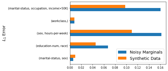
Remark 5: It is not surprising that the synthetic data enjoys lower error than the noisy marginals. Problem \ref{eq1} can be seen as a projection problem, and there is substantial theoretical [NTZ12] and empirical [LWK15, AAGK+19] evidence that solving this problem reduces error. Intuitively, the benefit arises due to the inconsistencies in the noisy observations that are resolved through the optimization procedure.
We can also use the synthetic data to estimate marginals we didn’t measure with the Gaussian mechanism. These estimates may or may not be accurate, it depends on the data and the marginal being estimated. For example, the error on the (sex, income>50K) marginal is around 0.02, while the error on the (education-num, occupation) marginal is about 0.5.
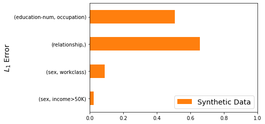
Remark 6: The fact that the synthetic data is not accurate for some marginals is not a limitation of the method used for Generate, but rather an artifact of what marginals were selected. Thus, it is clear that selecting the right marginals to measure plays a crucial role in the quality of the synthetic data. This is an important open problem that will be the topic of a future blog post.
Coming up Next
In this blog post, we focused on the Generate step of the select-measure-generate paradigm. For the next blog post in this series, we will focus on state-of-the-art approaches to the Select sub-problem. If you have any comments, questions, or remarks, please feel free to share them in the comments section below. If you would like to try generating synthetic data with MBI, check out this jupyter notebook on Google Colab!
-
The Generate step is a post-processing of already privatized noisy marginals, and therefore the privacy analysis only needs to reason about the first two steps. ↩
-
Here we assume that \( \mathcal{M} \) is a mechanism with a discrete output space. In practice, this is always the case because any mechanism implemented on a finite computer must have a discrete output space. For continuous output spaces, interpret the objective function as a log density rather than a log probability. ↩
-
For example, this worst-case behavior is realized if all 2-way marginals are measured. While this can be seen as a limitation of PGM, it is known that generating synthetic data that preserves all 2-way marginals is computationally hard in the worst-case. ↩
-
This idea was refined into RAPsoftmax in follow-up-work, which overcomes the latter issue, but does not resolve the non-convexity issue. ↩
-
These approximations were all developed concurrently, and systematic empirical comparisons between them (and PGM) have not been done to date. Some experimental comparisons can be found in [LVW21] and [MPSM21]. ↩
[cite this]