Welcome to ALT Highlights, a series of blog posts spotlighting various happenings at the recent conference ALT 2021, including plenary talks, tutorials, trends in learning theory, and more! To reach a broad audience, the series will be disseminated as guest posts on different blogs in machine learning and theoretical computer science. Given the topic of this post, we felt DifferentialPrivacy.org was a great fit. This initiative is organized by the Learning Theory Alliance, and overseen by Gautam Kamath. All posts in ALT Highlights are indexed on the official Learning Theory Alliance blog.

The second post is coverage of Shay Moran’s tutorial, by Kush Bhatia and Margalit Glasgow.

---

The tutorial at ALT was given by Shay Moran, an assistant professor at the Technion in Haifa. His talk focused on recent results showing a deep connection between two important areas in learning theory: online learning and differentially private learning. While online learning is a well-established area that has been studied since the invention of the Perceptron algorithm in 1954, differential privacy (DP) - introduced in the seminal work of Dwork, McSherry, Nissim, and Smith in 2006 [DMNS06] - has received increasing attention in recent years from both theoretical and applied research communities along with industry and the government. This recent interest in differential privacy comes from a need to protect the privacy rights of the individuals, while still allowing one to derive useful conclusions from the dataset. Shay, in a sequence of papers with co-authors Noga Alon, Mark Bun, Roi Livni, and Maryanthe Malliaris, revealed a surprising qualitative connection between these two models of learning: a concept class can be learned in an online fashion if and only if this concept class can be learned in an offline fashion by a differentially private algorithm.

The main objectives of this tutorial were to give an in-depth foray into this recent work, and present an opportunity to young researchers to identify interesting research problems at the intersection of these two fields. This line of work ([ALMM19], [BLM20]) - which has been primarily featured in general CS Theory conferences, including recently winning a best paper award at FOCS - introduced several new techniques which could be of use to the machine learning theory community. The first part of this article focuses on the technical challenges of characterizing DP learnability and the solutions used in Shay’s work, which originate from combinatorics and model theory. In the rest of this article, we highlight some of the exciting open directions Shay sees more broadly in learning theory.

Background: PAC Learning, Online Learning, and DP PAC Learning

We begin by reviewing the classical setting of PAC learning. The goal of PAC learning is to learn some function from a concept class \(\mathcal{H} \), a set of functions from some domain \( \mathcal{X} \) to \( \{0, 1\} \). In the realizable setting of PAC learning, which we will focus on here, the learner is presented with \( n \) labeled training samples \( \{(x_i, y_i)\}_{i=1}^{n} \) where \( x_i \in \mathcal{X} \) and \( y_i = h(x_i) \) for some function \( h \in \mathcal{H} \). While the learner knows the concept class \( \mathcal{H} \), the function \( h \) is unknown, and after seeing the \( n \) samples, the learner algorithm \( A \) must output some function \( \hat{h}: \mathcal{X} \rightarrow \{0, 1\} \). A concept class is PAC-learnable if there exists an algorithm \( A \) such that for any distribution over samples, as the number of labeled training samples goes to infinity, the probability that \( \hat{h} \) incorrectly labels a new random sample goes to 0. We will say that \( A \) is a proper learner if \( A \) outputs a function in \(\mathcal{H}\), while \( A \) is improper if it may output a function outside of \( \mathcal{H} \). More quantitative measures of learnability concern the exact number of samples \( n \) needed for the learner to correctly predict future labels with nontrivial probability.

DP PAC learning imposes an additional restriction on PAC learning: the learner must output a function which does not reveal too much about any one sample in the input. Formally, we say an algorithm \( A \) is \( (\varepsilon, \delta) \)-DP if for any two neighboring inputs \( X = (X_1, \cdots, X_i, \cdots, X_n) \) and \( X’ = (X_1, \cdots, X_i’,\cdots, X_n) \) which differ at exactly one sample, for any set \( S \), \( \Pr[A(X) \in S] \leq e^\varepsilon Pr[A(X’) \in S] + \delta \) . A concept class is DP PAC learnable if it can be PAC-learned by a \( (0.1, o(1/n)) \)-DP algorithm \( A \). That is, changing any one training sample \( (x_i, y_i) \) should not affect the distribution over concepts output by \( A \) by too much.

Online learning considers a setting where the samples arrive one-by-one, and the learner must make predictions as this process unfolds. 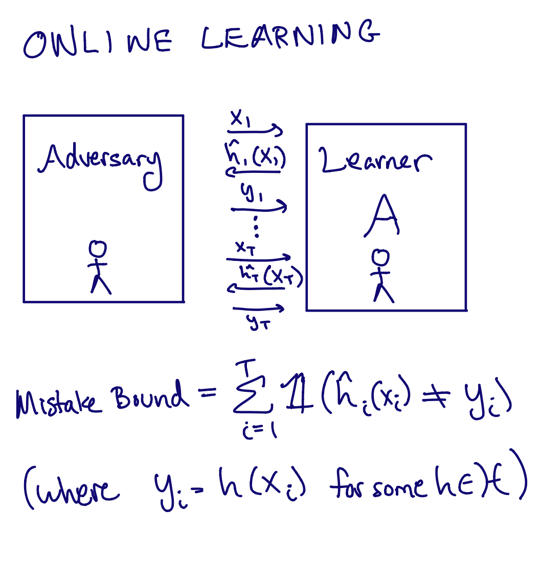Formally, in realizable online learning, at each round \( i = 1,\dots,T \), the learner is presented with a sample \( x_i\). The learner must predict the label, and then the true label \( y_i \) is revealed to the learner. The sequence of examples \( x_i \) and the labels \( y_i \) may be chosen adversarially, but they must be consistent with some function \( h \in \mathcal{H} \). The goal of the learner is to minimize the total number of mistakes made by round \( T \), also called the mistake bound. If there is a learner such that at \( T \rightarrow \infty \), the number of mistakes is \( o(T) \), we say that the class of functions \( \mathcal{H} \) is online learnable. Because of the adversarial nature of the examples, online learning is well known to be much harder than PAC learning, and is possible precisely when the Littlestone Dimension of the concept class is finite. Figure 1 below illustrates the definition of the Littlestone Dimension. One important PAC-learnable concept class which is not online learnable is the infinite class of thresholds on \( \mathbb{R} \): The set of functions \(\{h_t\}_{t \in \mathbb{R}} \) where \( h_t(x) = \textbf{1}(x > t) \).

Figure 1: The Littlestone dimension is the maximum depth of a tree shattered by \( \mathcal{H} \), where each node may contain a unique element from \(\mathcal{X}\). The tree is shattered if each leaf can be labeled by a function in \(\mathcal{H} \) that labels each element on the path to the root according to the value of the edge entering it. In this figure, we show how the set of thresholds on \( [0, 1] \) shatters this tree of depth 3.

It’s worth taking a moment to understand intuitively why learning thresholds might be hard for both an online learner and a DP learner. In an online setting, suppose the adversary chooses the next example to be any value of \( x \) in between all previously 0-labeled examples and all 1-labeled examples. Then no matter what label \( A \) chooses, the adversary can say \( A \) was incorrect. In a DP setting, a simple proper learner that outputs a threshold that makes no errors on the training data will reveal too much information about the samples at the boundary of 0-labeled samples and 1-labeled samples.

A Challenging Question

The journey to characterizing DP PAC learnability started soon after the introduction of DP, in [KLNRS08], where the concept of DP PAC learning was introduced. This work primarily considered the more stringent pure DP-learning, where \( \delta = 0\). This work established that any finite concept class could be learned privately by applying the exponential mechanism (a standard technique in DP) to the empirical error of each candidate concept. Using the exponential mechanism, the learner could output each function \( h \in \mathcal{H}\) with probability proportional to \( \exp(- \varepsilon(\# \text{ of errors h on the training data})) \). This was sufficiently private because the empirical error is not too sensitive to a change of one training sample. Later works [BNS14] combinatorially characterized the complexity of pure DP PAC learning in terms of a measure called representation dimension, showing that in some cases where PAC learning was possible, pure DP PAC learning was not. [BNSV15] further yielded lower bounds on the limits of proper DP PAC learning.¹
Both pure and proper DP learning though are significantly more stringent than improper DP learning, and proving lower bounds against an improper DP learner posed a serious challenge. Even the following simple-sounding question was unsolved:

Can an improper DP algorithm learn the infinite class of thresholds over [0, 1]? (*)

This question stands at the center of Shay’s work, which unfolded while Shay was residing at the Institute for Advanced Study (IAS) at Princeton from 2017 to 2019.² At the time, Shay was working on understanding the expressivity of limited mutual-information algorithms, that is, algorithms which expose little information about the total input. “If we were to have directly worked on this problem, I believe we wouldn’t have solved it,” Shay says. Instead, they came from the angle of mutual-information, a concept qualitatively similar to DP, but armed with a rich toolkit from 70 years of information theory. One of Shay’s prior works with Raef Bassily, Ido Nachum, Jonathan Shafer, and Amir Yehudayof established lower bounds on the mutual information of any proper algorithm that learns thresholds [BMNSY18], though this didn’t yet address the challenge presented by improper learners.

Unlike most lower bounds in theoretical computer science, proving hardness of learning the infinite class of thresholds on the line against an improper DP algorithm would require coming up with algorithm-specific distributions over samples. That is, instead of showing that one distribution over samples would be impossible to learn for all algorithms — in the way the a uniform distribution over the set in \(\mathcal{X}\) shattered by the concept class is hard to PAC-learn for any algorithm — they would have to come up with a distribution on \(\mathcal{X}\) specific to each candidate learning algorithm. Indeed, if the distribution was known to the learner, it was possible to devise a DP algorithm using the exponential mechanism (again!) which could learn any PAC-learnable concept class. Similar to the case of finite concept classes, here we can apply the exponential mechanism to some finite set of representative functions forming a cover of the concept class.

Uncovering a Solution

At the IAS, Shay met his initial team to tackle this obstacle: Noga Alon, a combinatorialist, Roi Livni, a learning theorist, and Maryanthe Malliaris, a model theorist. Shay and Maryanthe would walk together from IAS to their combinatorics class at Princeton taught by Noga and discuss mathematics. While Marayathe studied the abstract mathematical field of model theory, Shay and Maryanthe soon noticed a connection between model theory and machine learning: the Littlestone dimension. “There is applied math, then pure math, and then model theory is way over there,” Shay elaborates. “If theoretical machine learning is between applied math and pure math, model theory is on the other extreme.” This surprising interdisciplinary connection led them to use a result from model theory: a concept class had finite Littlestone Dimension precisely when the concept class had finite threshold dimension (formally, the maximum number of threshold functions that could be embedded in the class). This meant that answering (*) negatively was enough to show that DP PAC learning was as hard as online learning.

The idea for showing a lower bound for improper DP learning of thresholds came from Ramsey Theory, a famous area in combinatorics. Ramsey theory guarantees the existence of structured subsets among large, but arbitrary, combinatorial objects. A toy example of Ramsey Theory is that in any graph on 6 or more nodes, there must be a group of 3 nodes which form either a clique or an independent set. In the case of DP learning thresholds, the learning algorithm \( A \) is the arbitrary (and unstructured) combinatorial object. Ramsey Theory guarantees that for any PAC learner \( A \), there exists some large subset \( \mathcal{X}’ \) of the domain \(\mathcal{X}=[0, 1]\) on which \( A \) is close to behaving “normally”. The next step is to show that behaving normally contradicts differentially privacy. We’ll dig more technically into this argument in the next couple paragraphs. Note that we invent a couple definitions for the sake of exposition (“proper-normal” and “improper-normal”) that don’t appear in [BNSV15] or [ALMM19].

Let’s start by seeing how a simpler version of this argument from [BNSV15] works to show that proper DP algorithms cannot learn thresholds. Recall that in a proper algorithm, after seeing \( n \) labeled samples, \( A \) must output a threshold. To be a PAC learner, if exactly half of the \( n \) samples are labeled \( 1 \) (which we will call a balanced sample), \( A \) must output a threshold between the smallest and largest sample with constant probability. Indeed, otherwise the empirical error of \( A \) will be too large to even hope to generalize. This implies that for a balanced list of samples \( S = [(x_1, 0), \ldots ,(x_{n/2}, 0), (x_{n/2+1}, 1), \ldots ,(x_n, 1)] \) (ordered by \(x\)-value), there must exist an integer \( k \in [n] \) for which with probability \( \Omega(1/n) \), \(A \) outputs a threshold in between \( x_k \) and \( x_{k+1} \). We’ll say that \( A \) is \(k\)-proper-normal on a set \( \mathcal{X}’ \) if for any balanced sample \( S \) of \( n \) points in \( \mathcal{X}’ \), \( A \) outputs a threshold in between the \(k\)th and \(k+1\)th ordered samples with probability \( \Omega(1/n) \). For example, the naive algorithm that always outputs a threshold between the 0-labeled samples and 1-labeled samples is \(n/2\)-normal on the entire domain \([0, 1]\). Ramsey theory guarantees that there is an arbitrary large subset of the domain \([0, 1]\) on which \(A \) is \(k\)-proper-normal for some \(k\). (See Figure 2).

Figure 2: Ramsey’s Theorem guarantees a large subset \( \mathcal{X}’ \) on which \( A \) is \( k \)-proper-normal for some \( k \).

The second part of the argument shows that being \( k \)-proper-normal on a large set is in direct conflict with differential privacy. We show this argument in Figure 3 by constructing a set of \( n \) samples \( S^* \) on which \( A \) must output a threshold in many distinct regions with substantial probability.

Figure 3: A distribution showing the conflict between \(A \) being DP and \(k\)-proper normal. By DP, the behaviour of \(A\) on \(S^* \) must be similar to its behaviour on \(S_i\) for \(i = 1 \ldots \Omega(n).\) Namely, since \(S^* \) and \( S_i \) differ by at most two points, \( A(S^*) \) must output a threshold in \( I_i \) with probability \( p \geq (q - 2\delta)e^{-(2\varepsilon)} \) for each \( i \), where \( q \) is a lower bound on the probability that \( A(S_i) \) outputs a threshold in \( I_i \). Because \( A \) is \(k\)-proper-normal, \( q > c/n \), so \( p = \Omega(1/n) \). This yields a contradiction for \( m >1/p \) because \( A \) cannot simultaneously output a threshold in two of the intervals \( I_i \).

For the case of improper algorithms, Shay and his coauthors considered an alternative notion of normality, which we will term improper-normal. Recall that in this case the output \( A(S) \) of the learner on a sample \( S \) is any function from \( [0, 1] \) to \( \{0, 1\} \) and not necessarly a threshold. We’ll say that \( A \) is \(k\)-improper-normal on a set \( \mathcal{X}’ \) if for any balanced sample \( S = [(x_1, 0), \ldots, (x_{n/2}, 0), (x_{n/2 +1}, 1), \ldots, (x_n, 1)] \) of \( n \) points in \( \mathcal{X}’, \Pr[A(S)(w) = 1] - \Pr[A(S)(v) = 1] > \Omega(1/n) \) for any \( w \in (x_{k - 1}, x_k) \) and \( v \in (x_k, x_{k + 1}) \) in \( \mathcal{X}’ \setminus \{x_1, … x_n\} \). To PAC learn, A must be \(k\)-improper-normal for some \(k\) on any set of \(n + 1\) points. Applying the same Ramsey Theorem to a graph with colored hyperedges of size \(n + 1\) shows that there must exist an arbitrarily large set \( \mathcal{X}’ \) on which \( A \) is \(k\)-improper normal for some \( k \). A similar (but more nuanced) argument as before shows that a learner cannot be simultaneously private and \(k\)-improper-normal on some distribution over \( \mathcal{X}’ \).

For the last piece of the puzzle, showing the upper bound converse, Mark Bun, an expert in differential privacy at Princeton at the time, joined in. Beginning in the fall of 2019, Mark, Shay, and Roi worked out an upper bound that showed that any class with finite Littlestone dimension could be learned privately. Their technique introduced a new notion of stability, called global stability, which is a property of algorithms that frequently output the same hypothesis. Given a globally stable PAC learner \( A \), to obtain a DP PAC learner, one can run \( A \) many times and produce a histogram of the output hypotheses, add noise to this histogram for the sake of privacy, and then select the most frequent output hypothesis. The construction for the globally stable learner uses the Standard Optimal Algorithm for online learning as a black box - though the reduction is very computationally intensive and results in a sample complexity depending exponentially on the Littlestone Dimension. This reduction was improved in [GGKM20], where the authors gave a reduction requiring only polynomially many samples in the Littlestone dimension.

Outlook

Shay mentions that these results are only a first step towards understanding differentially private PAC learning. This work establishes a deep connection between online learning and DP learning, qualitatively showing that these two problems have similar underlying complexity. Recent works [GHM19] have gone a step further and established polynomial time reductions from DP learning to online learning under certain conditions. At the same time, Bun [B20] demonstrates a computational gap between the two problems: they exhibit a concept class which is DP PAC learnable in polynomial time, but no algorithm can learn it online in polynomial time and sample complexity.

An interesting question here is whether a polynomial time online learning algorithm implies a polynomial time DP learning algorithm? With regards to sample complexity, tighter quantitative bounds relating the sample complexity of DP learning to the Threshold dimension and the Littlestone Dimension, along with constructive reductions from DP learning to online learning are wide open. An interesting conjecture, also highlighted in the talk, is whether DP PAC learning and PAC learning are actually equivalent up to a \(log*\) factor of the Littlestone dimension? Solving this would mean that for most natural function classes, one need not pay a very high price for private learning as compared to PAC learning.

From a more practical perspective, studying such qualitative equivalences can lay the groundwork allowing one to use the vast existing knowledge in the field of online learning to design better algorithms for DP learning, and vice versa. Despite its abstractness, Shay believes this result still has significance for engineers: “If they want to do something differentially privately, if they already have a good online learning algorithm for this, maybe they can modify it,” Shay says. “It gives some kind of inspiration.”

From a broader perspective, Shay believes that discovering clean, beautiful mathematical models that are more realistic than the PAC learning model and understanding the price one pays for privacy in those models are important directions for future research. One model, highlighted in the tutorial by Shay is that of Universal Learning, introduced in a recent work [BHMVY21] with Olivier Bousquet, Steve Hanneke, Ramon van Handel and Amir Yehudayoff. This model considers a learning task with a fixed distribution of samples and studies the hardness of the problem as the number of samples \( n \to \infty \). This setup better captures the practical aspects of modern machine learning and overcomes the limitations of the PAC model, which studies worst-case distributions for each sample size.

And how should one go about identifying such better mathematical models? “Pick the simplest problem that you don’t know how to solve and see where that leads you”, says Shay. One should begin by trying to understand the deficiencies of existing learning models, by identifying simple examples which go beyond these existing models. For example, Livni and Moran [LM20] exhibit the limitations of PAC-Bayes framework through a simple 1D linear classification problem. Fixing such limitations can often lead one to discover better learning models.

---

Thanks to Gautam Kamath, Shay Moran, and Keziah Naggita for helpful conversations and comments.